Understanding Punching Shear
Part 1 - The Basics
1.1 Introduction
Two-way shear - also known as punching shear - is a force transfer mechanism between two-way slabs and its supporting columns1. It is prevalent in modern concrete construction because no one builds traditional beam-supported slab anymore. The preferred system in concrete highrises today is flat plates2- where the slab is supported directly on top of columns; no beams, no girders, just a smooth monolithic plate. The figure below illustrates the uniqueness of this approach vs. a more traditional system of intersecting beams.
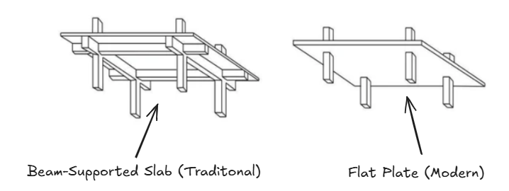
The traditional approach has mostly fallen out of favor because the presence of beams and girders results in deeper floors, more complicated formwork, more carpentry work, more labor, higher cost, and longer construction time. On the other hand, flat plates are much easier to construct (having a flat soffit), and much quicker to build3. Furthermore, shallower floor depths - through the course of 20+ stories - could mean an additional floor within the same building height constraint.
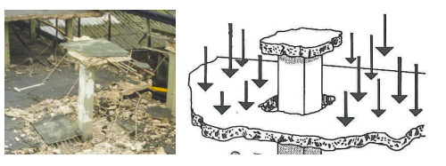
So what is the trade-off? The lack of supporting beams means less redundancy and high shear stress around the supporting columns. If improperly design, flat plates can fail suddenly without warning, often triggering progressive collapse. Below is an illustration of punching shear failure. The photo on the left is from the Piper’s Row Car Park collapse, which occurred in Wolverhampton, UK in the 1960s. Images like these keep engineers up at night.
1.2 Punching Shear
Let’s start with the basics and gradually introduce more nuance. In its simplest form, punching shear stress is simply equal to the force transferred to the column divided by the area of a theoretical failure plane around the column (i.e. \(V_u/A\)). This failure plane is technically an inverted truncated cone; however, ACI-318 allows the critical shear perimeter to be approximated as rectangular faces offset \(d/2\) from the column face (shown as red dashed lines in the figure below).
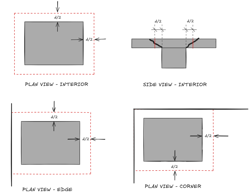
The total shear area is equal to the perimeter (\(b_o\)) multiplied by the slab depth (\(d\))4.
\[A_v = b_o d\]Therefore, punching shear stress, with negligible moment transfer, is simply the total force transferred to the column (\(V_u\)), divided by the shear area5. Notice I use lowercase \(v\) to denote stress, and uppercase \(V\) to denote force.
\[v_u =V_u/A_v\]1.3 Punching Shear With Moment
In practice, the simple equation above is only good for preliminary estimates. Concrete structures are monolithic after all. Moment transfers are always present, and can arise from unequal spans, uneven load distribution, uneven stiffness, and many other factors. It is unreasonable to assume zero moment transfer, especially at edge and corner columns.
To account for the effect of moment transfer, ACI-318 section 8.4.4.2.3 provides an equation that’s very similar to the combined elastic stress formulas (\(P/A + My/I\))6. The first term is what we have above, while the second term accounts for additional shear stress due to moment.
\[v_u = \frac{V_u}{b_o d} \pm \frac{\gamma_v M_{sc} c}{J_c}\]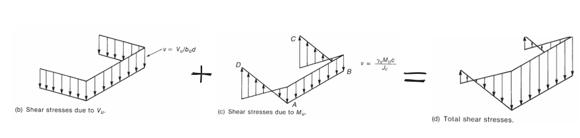
The illustration above is from the Macgregor Textbook 7, which is the main reference for almost everything in this article. Let’s go through the variables in the second term in detail:
Unbalanced Moment (\(M_{sc}\))
Unbalanced moment is simply moment transferred into the columns. Most FEM software will report this value directly. There are other methods for getting the unbalanced moment, such as applying coefficients to “statical moments”, but these methods are mostly outdated and no longer used in practice.8.
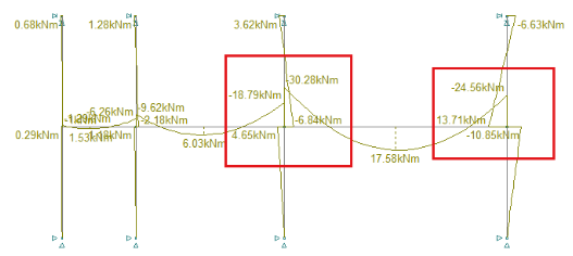
The word “unbalanced” hints at the notion that the floor wants to sag more on one side vs. the other - like an unbalanced seesaw. Unbalanced moments show up visually as a vertical offset in the moment diagram. Don’t be confused by this. Everything must be balanced in static equilibrium. Indeed, if we plot the moment diagram for the entire floor assembly, we see exactly where the unbalanced moment is going: into the columns9. Another point worth noting is that forces transferred to the column (\(\Delta M\)) is NOT the same as forces already in the column (\(M\)).
Unbalanced moment exists even if you have a completely regular slab system with equal spans and equal stiffnesses. This is because the building code requires “checker-boarding” live loads, which means some unbalanced moment will inevitable arise due to uneven loading. At exterior columns, unbalanced moment is always quite significant. Without continuity of slabs, 100% of the slab moment must be transferred.
Moment Transfer Ratio (\(\gamma\))
The unbalanced moment described above can transfer into the columns in two ways:
- Flexure within a limited transfer widths (\(\gamma_f\))
- Eccentric Shear (\(\gamma_v\))
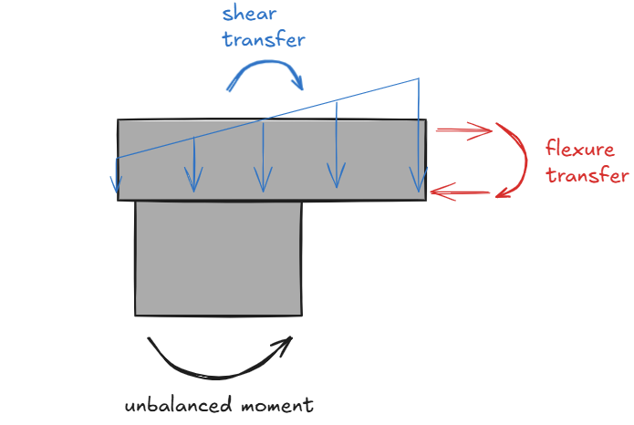
We use the Greek letter gamma (\(\gamma\)) to denote the percentage of moment transferred through each mechanism. Taken together, the two modes of transfer should add up to 100% (i.e. \(\gamma_v + \gamma_f = 1.0\)). The portion of moment transferred by eccentric shear (shown in blue above) is of interest to us because that is the portion that will increase shear stress. ACI-318 has equations for estimating \(\gamma_f\) and \(\gamma_v\) based on the critical shear section dimensions.
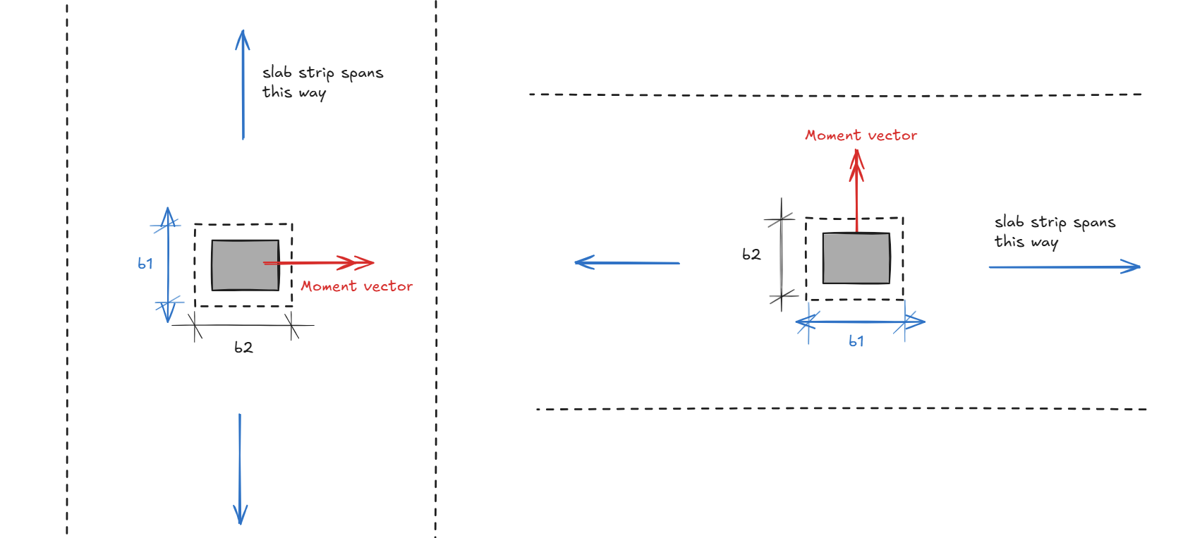
\[\gamma_f = \frac{1}{1+2/3\sqrt{\frac{b_1}{b_2}}}\] \[\gamma_v = 1 - \gamma_f\]In the equation above, \(b_1\) represents the critical perimeter dimension parallel to the slab span under consideration, whereas \(b_2\) is the perpendicular critical perimeter dimension. Here’s an illustration:
Distance From Shear Section Centroid (\(c\))
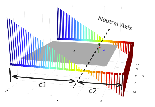
The variable \(c\) represents the distance from neutral axis to any fiber along the shear perimeter. Most of the time, we are interested in the fibers on the two extreme ends of the shear perimeter, like what’s shown below.
We can calculate the location of neutral axis (i.e. the centroid of the shear section) using the first moment of area formulas:
\[x_c = \frac{\sum xA}{\sum A} \mbox{ and } y_c = \frac{\sum yA}{\sum A}\]Please note the neutral axis doesn’t necessarily coincide with the column centroid - more on this in part 2. Furthermore, shear stresses due to \(M_{sc}\) usually acts in one direction only. Be careful and track signs (+ or -). The fiber furthest away from the neutral axis is NOT necessarily the governing fiber, you should check shear stresses at both ends. The governing fiber is usually the one where shear stresses due to gravity and unbalanced moment are additive.
“Property Analogous to Polar Moment of Inertia” (\(J_c\))
\(J_c\) is often referred to as a “section property analogous to polar moment of inertia”. There are many tables and formulas in design guides. Rather than providing a big table of formulas, let’s go through the derivations step-by-step. The calculation procedure is very similar to calculating section properties with the composite area method and parallel axis theorem, with a few idiosyncrasies that I will highlight. Before proceeding further, I’ll assume the reader has a basic understanding of second moment of area and related concepts (i.e. \(\bar{I} = \sum{ (I+Ad^2)}\)).
First, we divide the 3-D shear section into individual rectangular areas, then:
- For the areas highlighted green, calculate its \(I_x\) and \(I_y\) as well as any \(Ad^2\) terms. I call this the “web area”.
- For the areas highlighted blue, we calculate only its \(A d^2\) term and ignore the rest. I call this the “flange area”.
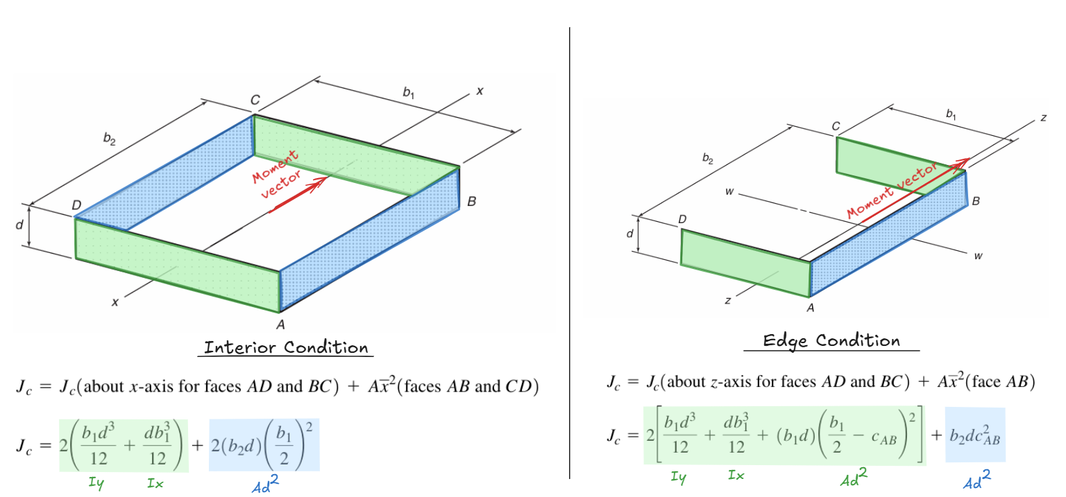
This is all a bit convoluted, to clarify, let’s derive the interior condition formula ourselves:
For the flange areas highlighted in blue, we only count the \(A d^2\) term. The area is equal to \(b_2d\), and the distance between the centroid of this area and the centroid of the overall section is equal to \((b_1/2)\):
\[Ad^2 = (b_2 d) (b_1/2)^2\]For the web areas highlighted in green, we will add up both the the \(I_x\) and \(I_y\) term. Since the centroid of green rectangle coincide with the centroid of the shear perimeter, we do not need to consider the \(A d^2\) term here (because \(d\) is 0). Recall that moment of inertia for a rectangular area is equal to \(I = bh^3/12\). Therefore:
\[I_x = \frac{d b_1^3}{12}\] \[I_y = \frac{b_1 d^3}{12}\]Putting all the pieces together, taking note that we have 2 “webs” and 2 “flanges”, we arrive at the same equation for interior condition as above:
\[J_c = 2(\frac{d b_1^3}{12}+\frac{b_1 d^3}{12}) + 2(b_2 d) (b_1/2)^2\]Alternatively, ACI 421.1R - Guide for Shear Reinforcement For Slabs presents a different formulation that is more generalized, and more conservative:
\[A_c = \sum L d\] \[J_{cx} = I_x = \sum \frac{L d}{3}(y_1^2 +y_1 y_2 + y_2^2)\] \[J_{cy} = I_y = \sum \frac{L d}{3}(x_1^2 +x_1 x_2 + x_2^2)\]In the equations above, a shear sections is composed of \(N\) straight segments, each segment defined by a start node \((x_1,y_1)\) and end node \((x_2, y_2)\) where the coordinates are relative to the shear section centroid; let \(L\) be the length of each segment, and let \(d\) be the slab depth.
Please note \(J_c\) per ACI 318 and \(J_{cx}, J_{cy}\) per ACI 421.1 are different in a subtle ways. We will discuss this difference in part 2.
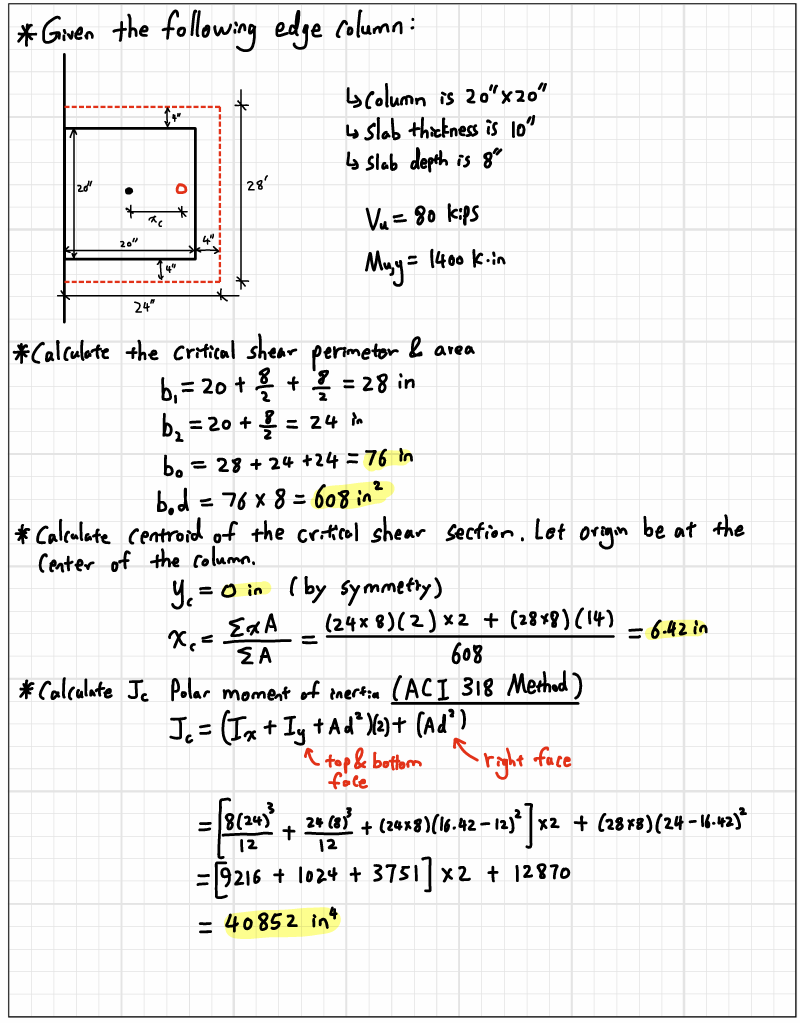
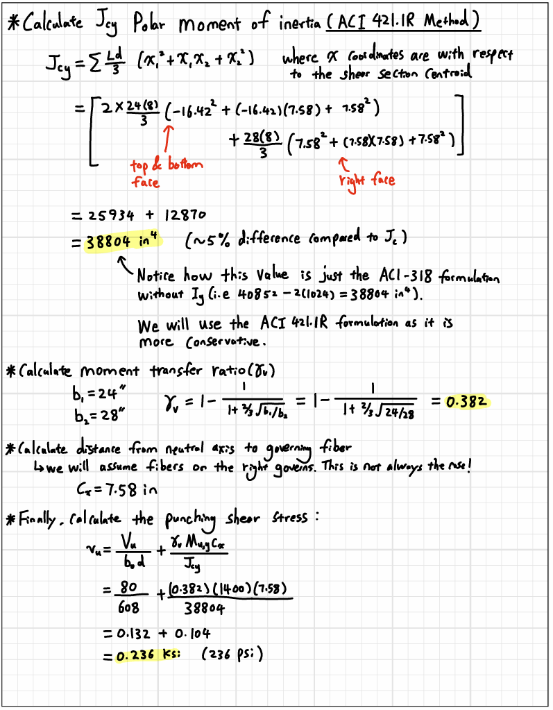
1.4 Example Problem
Now that we’ve covered all the important variables in the ACI 318 punching shear formulation. Let’s do an example calculation.
Part 2 - The Subtleties
“The devil lurks in the details”
2.1 Biaxial Unbalanced Moment
The astute reader may have noticed something peculiar about the formulations in Part 1. Why are we idealizing two-way slabs as two-dimensional frames? Two-way slabs are three-dimensional structures! What if there are unbalanced moment about both orthogonal directions?
ACI 318 code is vague about bi-axial moment for historical reasons. Before industry-wide adoption of FEM software, two-way slabs were designed using either the Direct Design Method (DDM), or Equivalent Frame Method (EFM), both of which required partitioning a three-dimensional slab system into series of two-dimensional frames. Slabs were designed one direction at a time in isolation, tediously along every gridline. With modern FEM software, it became trivial to find unbalanced moment about both axes, hence why it may seem strange to modern engineers why anyone would consider only “half” of the applied moment.
There’s ongoing debate on whether unbalanced moment should be considered one axis at a time, or both at the same time. A common line of argument is that calculating stress due to bi-axial moment will result in a maximum stress at a point, whereas all the experimental tests and thus code-based equations are based on the average stress across an entire face. According to the ACI committee 421 report in 1999 (ACI 421.1R-99), an overstress of 15% is assumed to be acceptable as stress is expected to distribute away from the highly stressed corners of the critical perimeter. However, this statement no longer exists in the latest version of the report (ACI 421.1R-20). I don’t think there is consensus yet. I’ll leave the engineering judgement to the reader. I would personally be as conservative as possible when it comes to punching shear.
Here’s the equation if we were to consider unbalanced moment about both axes.
\[v_u = \frac{V_u}{b_o d} \pm \frac{\gamma_{vx} M_{sc,x} c_y}{J_{cx}} \pm \frac{\gamma_{vy} M_{sc,y} c_x}{J_{cy}}\]ACI 318’s \(J_c\) should be used for single-axis unbalanced moment, whereas ACI 421.1R’s \(J_{cx}\) and \(J_{cy}\) should be used for bi-axial unbalanced moment. Although it is worth noting that \(J_{cx}\) and \(J_{cy}\) is always less than \(J_c\) so it’s always conservative to use ACI 421.1R’s formulation.
2.2 Slab Openings
According to ACI 318-19 22.6.4.3, If an opening is closer than \(4h\) to the critical shear perimeter, the shear perimeter (\(b_o\)) must be reduced which increases punching shear stress. To consider the influence of nearby openings, connect the corners of the opening to the column centroid, the portion of the shear section enclosed are considered ineffective. This is easier to explain with an illustration:
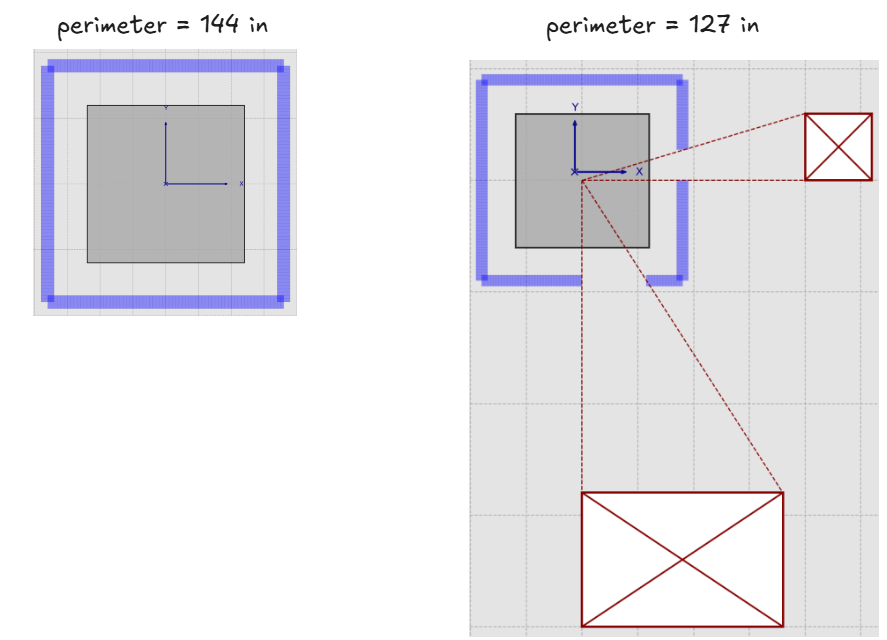
In practice, most engineers use some kind of CAD software to avoid doing the geometry puzzle. In addition to the perimeter reduction, there are two additional consequences that are often ignored:
- The addition of openings may shift the shear section centroid (see 2.4)
- The addition of opening may rotate the principal axes. For example, the section above on the right must be rotated 28 degrees to its principal orientation - where \(I_{xy}=0\) - otherwise equilibrium will not hold. (See 2.5)
2.3 Slab Edge Overhang
At edge or corner columns, the slab may cantilever far beyond the face of the column. At what point does it become an interior condition? According to ACI 318-19 22.6.4.1, the perimeter of the critical section shall be minimized. We will interpret this to mean that the overhang condition cannot provide more perimeter than if the column were on the interior. If we do the math, the limit works out to be \(c_2/2 +d\). Where \(d\) is the average slab depth, and \(c_2\) is the column dimension parallel to the slab edge. If the slab cantilevers longer than this limit, the edge condition becomes an interior condition.
\[\mbox{max overhang} = c_2/2 + d\]
Reality is more complicated. Ideally, engineers should avoid this grey area and ensure a clear distinction between edge and interior columns.
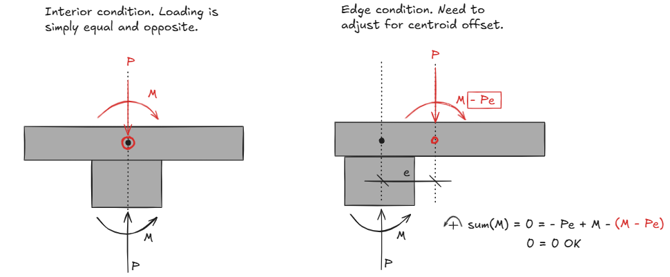
2.4 Shear Section Centroid Offset
The shear section centroid may not always coincide with the column centroid; this is illustrated graphically below.
Because of this eccentricity, ACI 421.1R highlights the existence of an additional moment:
\[M_{sc,x} = M_{sc,xO} + V_u (e_y)\] \[M_{sc,y} = M_{sc,yO} + V_u (e_x)\]However, this moment adjustment is not always applicable. The applicability depends on the FEM software you are using. Columns are typically modeled as one-dimensional stick elements without any physical dimensions; therefore, you’ll have to see how and where your software is reporting forces. Is it reporting moment at the face of the column? At the centroid of the column? At some distance d away from the column? Is the moment derived from integration of the slab stresses? Or is it derived from the column reactions?
2.5 Shear Section Principal Axes
In order for the beam flexural formulas - and by extension the ACI punching formula - to be applicable, the sections MUST be in its principal orientation. An alternative perspective is to say that the applied moment vector M must be resolved into components of the principal axes.
\[\sigma =M_xc_y/I_x +M_y c_x / I_y \Rightarrow \mbox{ this formula is only applicable if } I_{xy}=0\]For most symmetrical geometries, the principal axes is simply the horizontal (X) and vertical (Y) axes and no rotation is needed. However, there are sections - such as an L shape - that have diagonal principal axes. These situations are often referred to as unsymmetric bending. In short, where unsymmetric bending occurs, equilibrium is only guaranteed when the moment is applied with respect to the principal axes. To illustrate what I mean, In the figure below, I applied the exact same moment vector to a corner column. The only difference is the orientation of their x,y axes.
On the left, notice how the entire right face of the column has the same stress. This is expected as those fibers have the same \(c_x\) distance. Unfortunately, the resulting stress field is NOT in equilibrium.
On the right, we first resolve the moment into components of the principal axes \((x_p, y_p)\), and then apply the punching shear stress formula about these rotated axes. Notice the huge difference in shear stress between the two!
The degree of rotation required to get into the principal orientation can be found using those Mohr’s circle equations10. A nice shortcut is available for corner conditions with two equal length sides: in which case \(\theta_p = 45^o\).
\[\theta_p = \frac{1}{2} \arctan(\frac{2I_{xy}}{I_x - I_y})\]Distance from neutral axis to fiber (\(c\)) has to be with respect to the rotated axes. The major and minor moment of inertia about the principal axes is:
\[I_{xp,yp} = \frac{I_x + I_y}{2} \pm \sqrt{(\frac{I_x - I_y}{2})^2 +I_{xy}^2}\]The product of inertia term in the formula above can be determined using parallel axis theorem and properties of composite shapes:
\[I_{xy} = \int_A{xydA}= \sum (I_{xy,i} + A_i x_i y_i)\]A 45 degree rotation is still somewhat manageable, but it’s easy to see how it can quickly devolve into a tedious geometry puzzle at other angles.
2.6 Stud Rails
Steel reinforcements (stud rails) may be added to drastically increases a section’s shear capacity. However, we now need to verify the adequacy of two critical shear sections:
- The inner perimeter with increased capacity from stud rails.
- The outer unreinforced perimeter in the shape of a polygon.
The outer polygonal shear perimeter makes punching shear calculation very gnarly and tedious to do by hand - especially the geometric properties. Take this equation table from CRSI for example.
2.7 Polar Moment of Inertia - J
The parameter \(J_c\) was first introduced in a paper by Di Stasio and Van Buren (1960), the proposed analytical model was known as the eccentric shear stress model. The original formula had more factors in it but was subsequently simplified in ACI 318-71. The formula for punching shear has remained essentially unchanged since then.
ACI 318-19 defines \(J_c\) as a property “analogous to polar moment of inertia”. However, this terminology is misleading. It is perhaps better to think of \(J_c\) as purely an empirical constant rather than something theoretically rigorous. To understand why, recall from mechanics of materials some key equations:
\[\mbox{planar moments of inertia about X axis: } I_x=\int y^2dA\] \[\mbox{planar moments of inertia about Y axis: } I_y = \int x^2 dA\] \[\mbox{polar moment of inertia: } J = I_x + I_y\] \[\mbox{normal stress due to flexure: } \sigma = Mc/I\] \[\mbox{shear stress due to torsion: } \tau= Tr/J\]In material mechanics, we are taught that for any section, there can only be one polar moment of inertia (\(J\)) - which is used to calculate shear stress due to in-plane torsion (usually for circular shafts). On the other hand, a section has two planar moments of inertia (\(I_x\) and \(I_y\)) - which are used to calculate normal stress due to out-of-plane flexure.
The ACI 318 parameter \(J_c\) was born out of an attempt to fit our 3-D punching shear problem into equations that were meant for 2-D cross sections. We care about shear stress, but unbalanced moment is not a torsion because it’s applied out-of-plane, so do we use the flexural normal stress equation or the torsional shear stress equation?
The end result is a concoction that rhymes with both, but ultimately fits neither. \(J_c\) is suggestive of polar moment of inertia, but is used in a formula that resembles the flexural-normal-stress equation (\(\sigma=Mc/I\)). Despite being a polar moment of inertia, you can calculate two \(J_c\) values (\(J_{cx}\), \(J_{cy}\)), which means the mathematical relationship: \(J = I_x + I_y\) does not hold. Lastly, \(J_c\) becomes ill-defined for diagonal faces of a polygonal shear section.
Because of these drawbacks, ACI 421.1R - Guide for Shear Reinforcement For Slabs recommends using a slightly different formulation. The recommendation is basically to forget about \(J_c\), just calculate \(I_x\) and \(I_y\).
\[I_x = \int y^2dA \approx J_{cx}\] \[I_y = \int x^2dA \approx J_{cy}\]It turns out \(I_{x}\) and \(I_{y}\) approximates \(J_{cx}\) and \(J_{cy}\) very well. The former is usually around 95% of the latter, and since \(J_c\) is on the denominator, using the ACI 421.1R equations will always be more conservative. In effect, we are discarding the weak axis \(I_y\) term from the web areas (the one where slab depth is cubed), and end up just calculating a planar moment of inertia.
Rather than calculating the integral by hand, we have two options. The first is to use the method of composite shapes and parallel axis theorem. The first term is calculated using the MOI equation for a rectangle: \(bh^3/12\). For the “web area”, b = the slab depth and d = shear perimeter length, and for the “flange area”, b = shear perimeter width and d = 0.
\[I_x = \sum (I_{xi} + A_i d_i^2)\] \[I_y = \sum (I_{yi} + A_i d_i^2)\]Alternatively, we can use the handy formulas provided in ACI 421.1R. Let a shear section be composed of \(N\) straight segments, each segment is defined by a start node \((x_1,y_1)\) and end node \((x_2, y_2)\) where the coordinates are relative to the shear section centroid; let \(L\) be the length of each segment, and let \(d\) be the slab depth. The ACE 421.1R equations for J are shown below:
\[I_x= \sum \frac{L d}{3}(y_1^2 +y_1 y_2 + y_2^2)\] \[I_y = \sum \frac{L d}{3}(x_1^2 +x_1 x_2 + x_2^2)\]Let’s derive the formulas above ourselves. A single segment of a multi-segment shear perimeter is illustrated below.
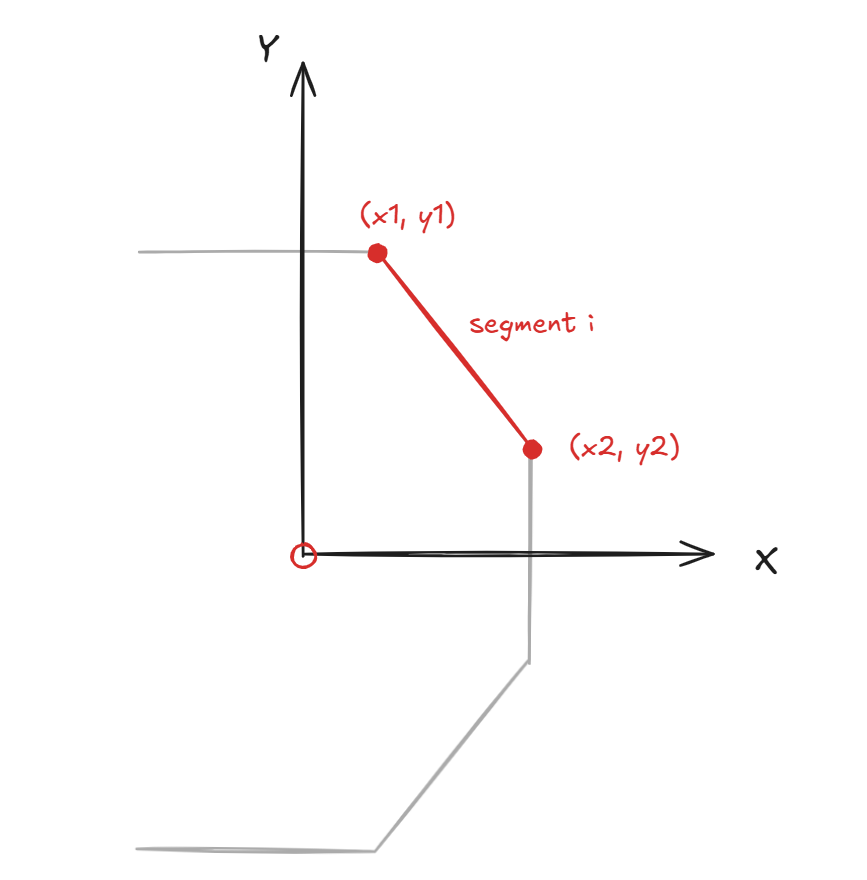
If a shear section is composed of only vertical or horizontal segments, we can take advantage of the parallel axis theorem without solving any integrals. But it gets a little more complicated when diagonals are present. To get the right answer, we will need calculate the line integral of individual segments, then sum the contribution of all segments.
For brevity, I will derive the formula for \(I_x\) only. The derivation for \(I_y\) is exactly the same just with x and y swapped. For a single straight segment:
\[I_{xi} = \int_c y^2dA\]A straight line segment i starting at \((x_1, y_1)\) and ending at \((x_2, y_2)\) can be parameterized as:
\[x = x_1 + t(x_2-x_1) \qquad \mbox{where} \qquad 0\leq t \leq 1\] \[y = y_1 + t(y_2 - y_1) \qquad \mbox{where} \qquad 0\leq t \leq 1\]Furthermore, we can simplify the differential arch length (for a straight segment) as:
\[ds = \sqrt{(\frac{dx}{dt})^2 + (\frac{dy}{dt})^2} dt\] \[\frac{dx}{dt} = (x_2-x_1)\] \[\frac{dy}{dt} = (y_2-y_1)\] \[ds = \sqrt{(x_2-x_1)^2 + (y_2-y_1)^2} dt\] \[ds = L dt\]The differential area is equal to the slab depth (\(d\)) multiplied by \(d_s\)
\[dA = ds \times d = (Ld) dt\]Substitute the equations above into our original integral:
\[I_{xi} = L d \times \int_0^1 (y_1 + t(y_2-y_1))^2 dt\]Expand terms:
\[I_{xi} = Ld \times \int_0^1 y_1^2 + 2y_1t(y_2-y_1) + t^2(y_2-y_1)^2 dt\]Solving the definite integral gets us:
\[I_{xi} = Ld \times (y_1^2t \rvert_0^1 + \frac{t^2 2y_1(y_2-y_1)}{2} \rvert_0^1 + \frac{t^3 (y_2-y_1)^2}{3} \rvert_0^1)\] \[I_{xi} = Ld \times ((y_1^2) + (y_1(y_2-y_1)) + \frac{1}{3}(y_2^2 - 2y_1y_2 + y_1^2))\]Do some simple algebra:
\[I_{xi} = Ld \times ((y_1^2) + (y_1y_2 - y_1^2) + (\frac{1}{3}y_2^2 - \frac{2}{3}y_1y_2 + \frac{1}{3}y_1^2))\] \[I_{xi} = Ld \times ( \frac{3}{3}y_1y_2 + \frac{1}{3}y_2^2 - \frac{2}{3}y_1y_2 + \frac{1}{3}y_1^2)\] \[I_{xi} = Ld \times ( \frac{1}{3}y_1y_2 + \frac{1}{3}y_2^2 + \frac{1}{3}y_1^2)\] \[I_{xi} = \frac{Ld}{3}(y_1^2 +y_1y_2 + y_2^2 )\]Remember the term above is the contribution of a single straight segment. Sum the contribution of all segments to get \(I_x\).
\[I_x = \sum \frac{Ld}{3}(y_1^2 +y_1y_2 + y_2^2 )\]Part 3 - Python Library
3.1 Introduction
wthisj is a python package I developed for punching shear calculations. It incorporates all of the nuances we’ve discussed above and more. The name stands for “what the heck is j?”, which was the original motivating question for why I started my deep dive on punching shear. The package - along with all of its source code - is available on Github.
I was motivated to make this tool when I noticed the interesting similarity between punching shear calculation, bolt force calculation, and welded group calculations, namely: they can all be categorized as utilizing the elastic method. The unifying theme between all three projects is that a force or stress field varies linearly, emanating from zero at some neutral axis, outwards to the extreme fiber/anchor/bolt/weld.
The entire package is essentially one .py file that defines a PunchingShearSection class with around 2,000 lines of code. If you follow me with my other projects, you’ll see the similarity with fiberkit, ezbolt, ezweld, ezanchor right away. In fact, I sometimes feel like I’m making the exact same project over and over just with a different vocabulary.
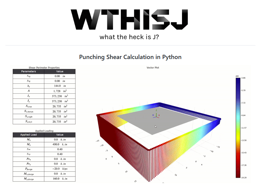
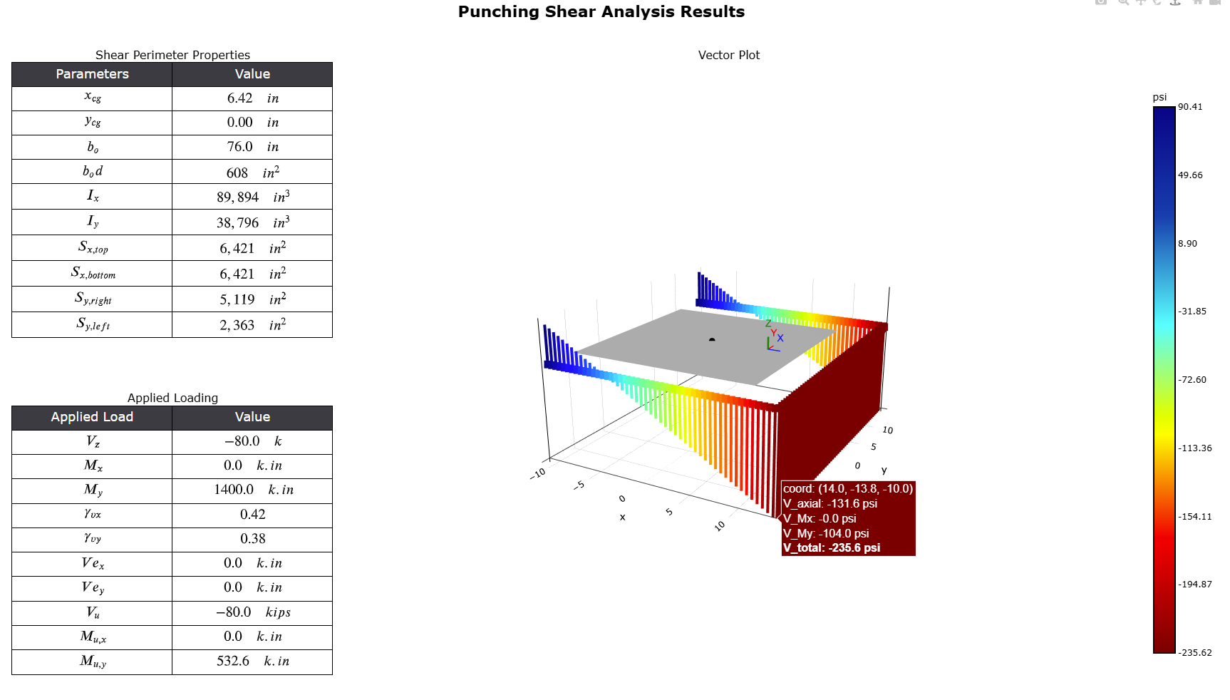
Here’s the same output from wthisj:
import wthisj
# define a punching shear section
column1 = wthisj.PunchingShearSection(col_width = 20,
col_depth = 20,
slab_avg_depth = 8,
condition = "W",
overhang_x = 0,
overhang_y = 0,
studrail_length = 0)
# solve
results = column1.solve(Vz = -80, Mx = 0, My = 1400, consider_ecc=False)
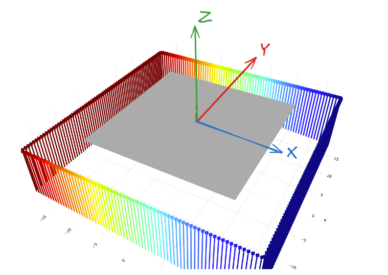
# plot results
column1.plot_results_3D()
The intent of this blog is to provide additional background on wthisj. If you are interested in how to install and use the tool, or the documentation, please refer to the GitHub Repo. With this post, I would like to provide additional context for some of the important decisions I had to make. Assumptions and simplifications are always necessary, and I will outline them here - along with some commentaries.
3.2 Numerical Approximation of J
I’ve outlined two methods for computing J above:
- ACI 318 method which calculates \(J_{cx}\) and \(J_{cy}\)
- ACI 421.1R method which calculates \(I_x\) and \(I_y\).
My preference is to use the latter because it’s both more conservative and more generalizable; however, rather than using the line integral equations presented above, wthisj uses numerical approximation to determine \(I_x\) and \(I_y\) by discretizing the shear perimeter into tiny 0.5 inch fibers, each fiber has an infinitesimal area (dA) which is then summed to approximate the integrals.
\[I_x = \int_A y^2 dA \approx \sum y_i^2 A_i\] \[I_y = \int_A x^2 dA \approx \sum x_i^2 A_i\]The default fiber size is usually accurate enough, but you can reduce the fiber size further by changing the PATCH_SIZE argument when initializing a PunchingShearSection() object.
3.3 (N, S, W, E) For Different Conditions
Three support conditions are possible in two-way slabs: (1) Interior, (2) edge, and (3) corner. Rather than fixing the position of slab edge, I want to make the visualization fully flexible and interactive. In other words, turn three conditions into nine. Unfortunately, this tripled the amount of work I had to do for parametrically generating line works in the plots. Nevertheless, my sense is that it’s worth it to be able to visualize exactly what you want to model - without mirroring or rotating it in your head.
At first, I used Matplotlib’s legend alignment strings: "upper right", "upper left", "lower center", etc.... But this convention grated me and I thought it was often confusing. Is it middle or center? Is it upper or top? Then it occurred to me that I could use the cardinal directions on a compass!
- Interior condition:
"I" - Edge condition:
"W", "E", "N", "S" - Corner condition:
"NW", "NE", "SW", "SE"
3.4 Adding Openings
ACI 318 describes how shear perimeter may be made ineffective in the presence of nearby openings. This is easy enough to understand geometrically, but quite hard to describe with words. Here’s the exact wording in ACI 318: “the portion of \(b_o\) enclosed by straight lines projecting from the centroid of the column, concentrated load or reaction area and tangent to the boundaries of the opening shall be considered ineffective”. Yea… Quite confusing until you see the graphics. In practice, I don’t know anyone who actually does this geometry puzzle by hand. Did you know you can calculate section properties in AutoCAD or BlueBeam?
I was utterly lost on how to implement this until I reframed the problem in polar coordinates, then it became trivial. The location of every fiber gets converted from \((x,y)\) to \((r, \theta)\). Each opening has four vertices, so I can loop through them to find a “\(\theta\) deletion range”. Every fiber that falls within the \(\theta\) deletion range gets removed. The benefit of numerical approximation and fiber discretization becomes clear here. The implementation of openings would have been much harder if I went with the line integral approach. atan2() again makes an appearance and makes me happy.
You can add an arbitrary number of rectangular openings in wthisj with the PunchingShearSection.add_opening(xo, yo, width, depth) method. A warning will be printed to console if the openings is further than 4h away because the specified opening can be ignored per ACI 318.
3.5 What about Punching Shear Capacity?
Adding a module for shear capacity calculation would have been simple enough. Here’s the equation for concrete capacity - it’s the minimum of the three equations below 11:
\[v_{c1} = (4) \lambda_s \lambda \sqrt{f'_c}\] \[v_{c2} =(2 + 4/\beta) \lambda_s \lambda \sqrt{f'_c}\] \[v_{c3} =(2 + \frac{\alpha_sd}{b_o}) \lambda_s \lambda \sqrt{f'_c}\]And here’s the equation for stirrup or stud rail capacity:
\[v_s = \frac{A_v f_{yt}}{b_o s}\]Maybe I’ll implement this in a future release. There are two reasons why I did not:
(1) I ran out of energy and momentum - and in all honesty I got bored. I thought this project would take me at most two weekends. It ended up taking 3 months, and I’m still writing about it 9 months later. My opinion is that calculating demand is theoretically more interesting. I’ll leave calculation of capacity as an exercise for the reader for now. If I do implement it in the future, it would be a separate method entirely uncoupled from the main workflow so as to avoid cluttering the init arguments.
(2) I am wary of providing both capacity and demand, especially for something as critical as punching shear. My sense is that providing both demand and capacity encourages users to take everything as gospel and trust wthisj as a black box. Please don’t. I work on these projects in a cafe in Fremont with terrible coffee and WIFI - often after a long day of work when I have very few brain cells to spare. This is not enterprise software.
3.6 Sign Convention
The figure below shows the sign convention in wthisj. It’s pretty standard right-hand convention.
When I specify Vz, Mx, My in wthisj, I am NOT referring to the column reactions. Instead, I am referring to an equivalent set of nodal force/moment that has the same effect as the external forces that are applied on the slab - which is equal and opposite to the column reactions. I hope I don’t confuse anyone. What I am getting at is that there aren’t actually concentrated force/moment at the slab-column joint. With the current convention, a downward force (-Vz) produces shear stress arrows that also point downwards, which I felt was the most natural.
An alternative perspective is to considerVz, Mx, My as forces on the underside of the column. With this convention, the upward internal force on the underside of the column produces shear stress on the perimeter that is in equilibrium and thus points downwards. I suspect most people don’t think of punching shear this way. I actually implemented this convention initially and it was very confusing.
Footnotes
-
Punching shear is also relevant in the design of footings; however, it’s usually less critical because footings tend to be thicker than slabs. The design equations are one and the same. To see the resemblance, just flip the column-to-footing free body diagram upside down. ↩
-
If column caps or drop panels are present, then the slab system is called flat slab. ↩
-
Concrete high-rises on the East Coast, especially residential apartment buildings, often utilize flying forms to further accelerate project timeline, and reduce the cost of formwork and labor. ↩
-
Slab depth is measured from the extreme compression fiber to the tension rebar centroid. It is different depending on which orthogonal rebar direction you are looking at. For design purposes, it is common to take the average depth of the two-orthogonal rebar directions ↩
-
Concrete design is very empirical which is why we only care about the average shear stress (V/A) ↩
-
It should be noted that although there is a \(\pm\) sign for the second term, unbalanced moment could sometimes be one-directional. Care should be taken in tracking the sign of the unbalanced moment. ↩
-
Irrelevant tangent: I absolutely love this textbook. Dr. MacGregor is my engineering hero and it’s only a bonus that he is also a fellow Canadian. ↩
-
In the past, unbalanced moment was derived using moment distribution coefficients of Direct Design Method (DDM), or simplified models of Equivalent Frame Method (EFM). Both methods are outdated and no longer used. Modern two-way slab design is usually done with the help of finite-element method (FEM) models. To get the best result from FEM, the engineer should make sure flexural stiffnesses of all connecting members are modeled accurately - including stiffness modifiers to account for cracking. ↩
-
Although tempting, it is erroneous to model a slab strip as a continuous beam with pin supports. Concrete columns have flexural stiffnesses and will attract moment (thus producing the vertical offset in the slab moment diagram). A more appropriate model would include the columns as well - thus turning a continuous beam model into a 2D frame model. The only situation where columns won’t attract any moment is If the column-slab joints remain horizontal (i.e. zero rotation). Another interesting behavior in this common 2D frame breakout model is that the upper column is in tension! ↩
-
If \(I_x = I_y\), then \(\theta_p = 45^o\). ↩
-
This punching shear capacity equation must be modified in many jurisdictions. The international Code Council published a report (ESR-2494) which concluded that 4sqrt(f’c) must be reduced to 1.5sqrt(f’c) More info here. ↩