Primer: Surveying Principles
“Primers” are my personal notes on various technical topics in structural engineering. Building codes are dense and voluminous, sometimes written in legalese rather than in sentences that can be easily understood. I write these “Primer” so I can gather, organize, and condense technical topics I encounter as an engineer. Please understand I made these for myself. Reader discretion is advised. No warranty is expressed or implied by me on the validity of the information presented herein.
- 1.0 California Surveying Law
- 2.0 Horizontal Measurements - Distance
- 3.0 Vertical Measurements - Elevations
- 4.0 Angle Measurements
- 5.0 Error Analysis and Distribution
- 6.0 Traverses
- 7.0 Topography
- 8.0 Route Surveying
- 9.0 Construction Staking
- 10.0 Photogrammetry
- Appendix: Miscellaneous Stuff
This is my study note which summarizes the content of Paul A. Cuomo’s “Surveying Principles for Civil Engineers” textbook. I highly recommened getting a physical copy, as it would be prudent for you to have it during the exam. Amazon Link
1.0 California Surveying Law
1.1 Types of Surveys
- Cartographic - rough hand sketches
- Boundary - property lines
- Geodetic - planetary wide perspective. Shape of the earth.
- Hydrographic - underwater land characteristic (existing body of water)
- Topographic - land elevation and objects. Conducted fairly early on prior to construction documents
- Route - highways, pipes (parallel and perpendicular measurements)
- Construction - field control during construction with stakes
- As-built - conducted after construction for record-keeping (final survey)
- Control - establish location of benchmarks
1.2 Survey Party
- Party chief - team leader
- Instrument person - often note keeper as well
- Rod person - holds rod plumb
- Chain persons - pair stretching tape between them
- Stake setter - drives stakes into ground per instrument or rod person
1.3 California Law
- Professional Land Surveyors Act
- Defines licensure requirements and roles of a surveyor
- Professional Engineers Act
- Defines licensure requirements for civil engineer and their allowed role
- Subdivision Map Act
- Defines procedure for boundary surveys (property lines) and how they are recorded by local municipality
- Parcel map = large parcel of land divided into (4) or less divisions
- Subdivision Map = large parcel of land divided into (5) or more divisions. AKA final map.
- Tentative Map - before developers submit their plans. Preliminary maps
- Licensed surveyor and Civil Engineer licensed BEFORE 1982 can do everything
- Civil engineer registered after 1982 CAN perform:
- contour surveys (aerial survey, topographic)
- survey of fixed work
- tunnel survey
- tentative maps
- Civil engineer registered after 1982 CANNOT perform:
- geodetic surveying (taking into account Earth’s curvature)
- cadastral surveying (records of property lines)
- survey for land division
- determine position of anything that establishes a property line
- Basically any sort of benchmark setting
2.0 Horizontal Measurements - Distance
2.1 Basic Trigonometry
- Vertical angle = angle with respect to horizontal line (\(\alpha\)). Think of it as a projection of our vector onto the horizontal line.
- Zenith angle - angle with respect to vertical line (\(z\)). Note you can use angle greater than 90 degrees directly because sin(z) = sin(90+z)
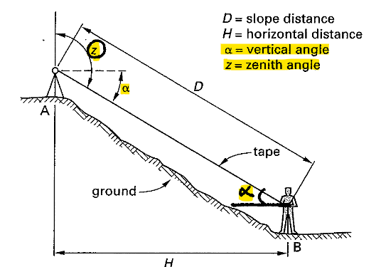 Figure 1: Horizontal Measurement Trigonometry
2.2 Taping and Chaining
- Taping and chaining involves two people measuring horizontal distance with Gunter’s chain (66 ft) or a steel tape. Try to measure horizontal distance directly without using any trigonometry (use a plumb bob for leveling)
- Here are some useful unit conversions:
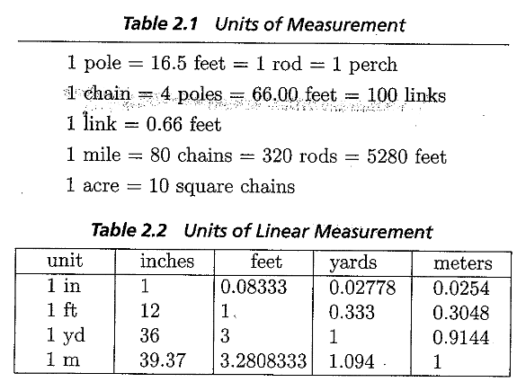 Figure 2: Common Unit Conversion
- 1 m = 3.28 ft
- 1 mile = 5280 ft
- 1 hectare = 2.472 acre
- 1 acre = 43560 ft^2
- 1 cubic yard = 27 ft^3
- There are three types of tapes: 1.) add tape, 2.) cut tape, and graduated tape. Their main difference is how the last feet is measured and calibrated (see figure below for an illustration. The rear chain-person holds the roll of tape. The forward chain-person holds near the zero mark.
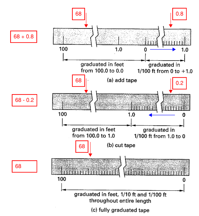 Figure 3: Different Type of Tape
- Temperature correction can be applied with the following equation. Let c = the correction amount. To = standard temperature = 68o>F unless otherwise noted.
- If T > To, the tape is hot and expanded which reads smaller, c is positive, real distance is actually larger
- If T < To, the tape is cold and contracted which reads bigger, c is negative, real distance is actually smaller
- Tape Sag Adjustment (always negative - actual length is shorter)
- w = weight of tape (lbs/ft or kg/m)
- P = pull force (lbs or kg)
- Don’t forget to divide by length (lbs/ft units!)
- Tape Pull Adjustment
- Po = standardized pull tension (usually around 15 lbs)
- A = cross section area of tape
- E = elastic modulus of steel (30 000 000 psi)
- When tape is measured at an incline. Make sure to correct for S, before calculating H
- Pay attention to units for the pull adjustment! Denominator can stay in inches because in^2 and psi cancels out
- For distance measurements exceeding tape length, need to add the adjustment from all measurements. For example, 450 ft, we will have (4) adjustment with 100 ft and (1) adjustment with 50 ft
2.3 Stadia Measurement
- Measuring distance with a lens w/ cross-hair and a rod. Distance can be indirectly deduced by reading the gap between cross-hair. Usually K = 100 ft and C is 0 ft unless otherwise noted.
- I is the crosshair reading as illustrated below:
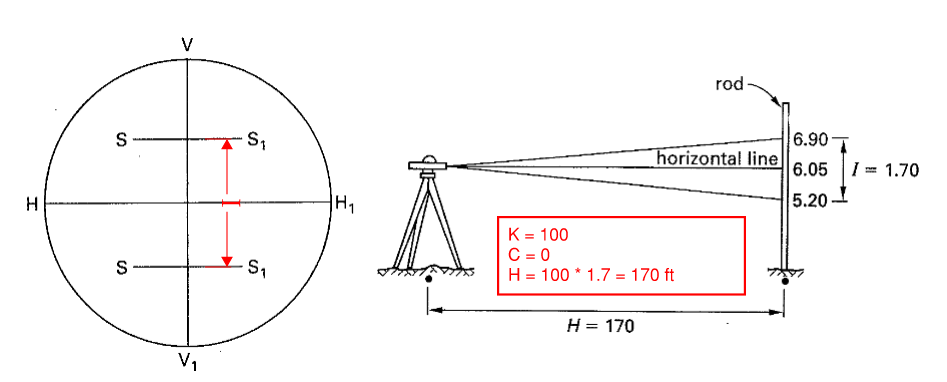 Figure 4: Stadia Cross Hair
- Very rare for reading to be level, more often you the scope is slanted and need to adjust measurements. Referring to the figure below:
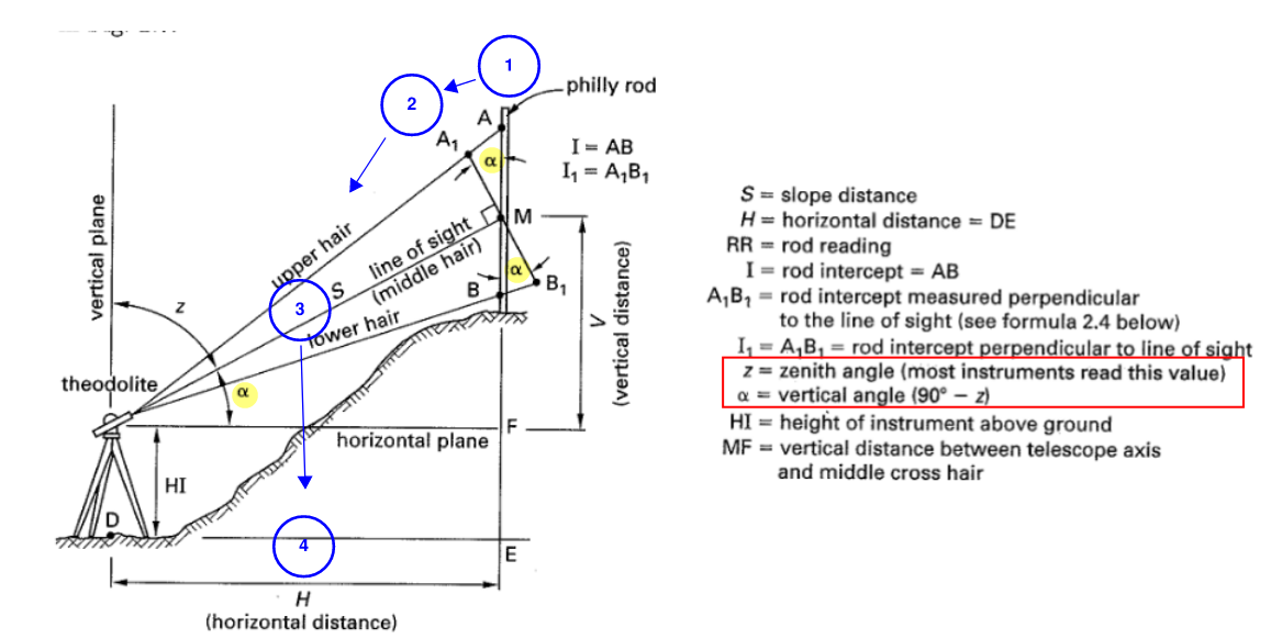 Figure 5: Inclined Stadia Measurement
- Reading line AB = I, which is longer than actual because slanted scope
-
Convert to the effective rod intercept by first determining the vertical angle. Note how the vertical angle corresponds in the figure above (\(\alpha\))
\[I_1 = I \cos(\alpha)\] -
Now the actual slanted distance (S) can be determined as we’ve shown before:
\[S = K I_1 + c = KI \cos(\theta) + c\] -
Finally let’s convert to horizontal and vertical distance. Note vertical distance is to center of rod reading.
\[H = S \cos(\alpha) = (KI \cos(\alpha) + c) \cos(\alpha)\] \[V = S \sin(\alpha) = (KI \cos(\alpha) + c) \sin(\alpha)\]
2.4 Electronic Distance Measuring (EDM) and Total Station
- EDM is essentially the high-tech version of stadia that is superior all around. Distance is measured by measuring wavelength of light as it is reflected. Occasionally, some error adjustment is required:
- Constant prizm offset. Reduce distanced measured by 30 mm to 40 mm (because of internal reflector distance)
- Varying atmospheric pressure adjustment (measured in ppm)
- Total station is the even more advanced version that allows for measurement of all distances and angles. No need to take notes when you have a total station.
3.0 Vertical Measurements - Elevations
3.1 Conceptual Stuff
- All elevation is measured with respect to a datum. In the US, that datum is based on the Mean Sea Level 1929 Adjustment (MSL29) and was updated to NGVD 88
- Here are some commonly used terminologies:
- leveling circuit - our instrument which has a telescope for rod readings. Often rotation is restricted to only vertical axis (i.e. always horizontal)
- (RR) rod reading
- (HI) instrument height - usually refers to elevation at sightline. But may also refer to height of equipment itself
- (BS) backsight - RR at the previous point of measurement. associated with plus (+)
- (FS) foresight - RR at the next point of measurement. associated with minus (-)
- (BM) benchmark - a location where we know the exact elevation (serves as control and error correction)
- (TBM) temporary benchmark - not official, usually used by individuals for temporary purposes
- (TP) turning point - point whose elevation is determined prior to moving the level
- Our instrument does not have to be placed in line of FS and BS (rotating 180 degree) each time. But our equipment should always be set up with equal distance to BS and FS to minimize curvature, collimation, and refraction errors. Having equal distance means the error could balance out.Curvature error arises because the surface of Earth is curved, but our line of sight is straight.
- If the above is not possible (say that places our instrument in the middle of a river), then use reciprocal leveling
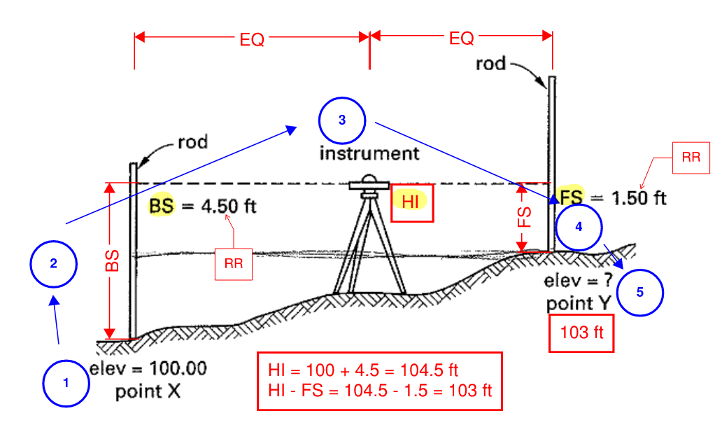 Figure 6: Leveling Instrument
Referring to the figure above, the procedure for leveling is as follows:
- We know elevation at point X is 100 ft
- From RR of BS, we read 4.5 ft
-
=> 100 + 4.5 = 104.5 ft is the elevation of HI
\[HI = elev_{BS} + BS\] - Now rotate to the FS, we read RR of FS as 1.5 ft. Subtract this value to get elevation of FS.
-
=> 104.5 - 1.5 = 103 ft is the elevation at Y
\[elev_{FS} = HI - FS\] - Move instrument, FS becomes the new BS, repeat until done
- Precise Leveling - high order of accuracy. Used to furnish low-order work. Covers large area. More precise equipment is used.
3.2 Indirect Leveling With Stadia
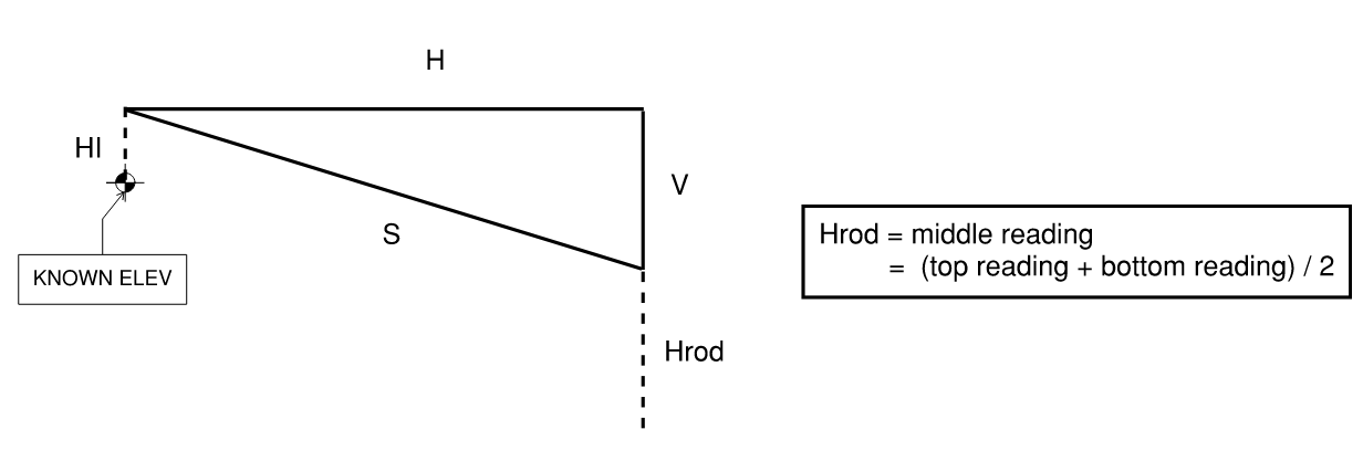
- Use stadia as we have seen in the last chapter, but calculate “V” this time. Then add/subtract by given elevation
- Often we need to adjust by add/subtracting rod and instrument height:
3.3 Leveling Rod
- Rods can extend up to 13 ft, with 0 at the base. There are two types:
- self-reading rod - Philadelphia rod (most popular)
- self-reducing rod - Lenker rod. No notes need to be taken. Set zero at HI. Value increases from top to bottom
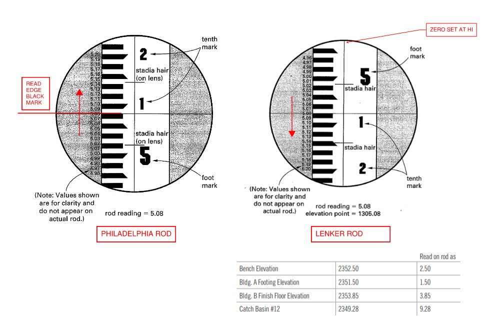 Figure 7: Type of Leveling Rod
3.4 Direct Leveling Note Example
Here is a sample note taken from the field. Note the sequence of calculation and how BS is associated with (+), and FS is associated with (-). Also note the summation check at the end to ensure no adjustment is needed.
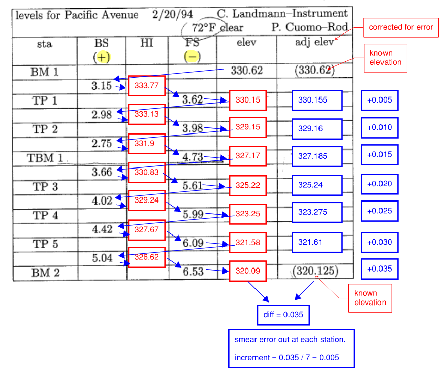 Figure 8: Leveling Note + Error Correction
Negative (-) error means too short. If the summation above does not calculate out, we need to smear the error in the “adjusted elevation column” as shown above.
3.5 Profile or Cross-Section Leveling
Involves obtaining elevation along a perpendicular line (used to determine a cross-section). The surveying note will now have a new column for side shots (SS)
\[elev_{SS} = HI - SS\]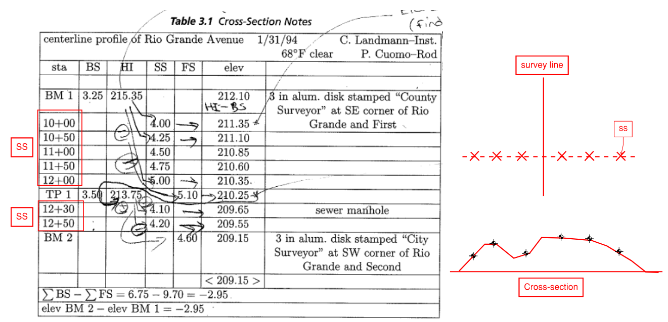 Figure 9: Profile Leveling
Note we can skip the intermediate SS when calculating TP1. Cannot skip if there is a BS recording
3.6 Reciprocal Leveling
Occurs when instrument cannot be placed equi-distance between FS and BS (such as in the middle of a river). We are essentially averaging out the error.
Calculate ELEV with instrument 1, calculate ELEV with instrument 2. Average the results.
 Figure 10: Reciprocal Leveling
4.0 Angle Measurements
4.1 Conceptual Stuff
- Three types of angle measurements. Internal and exterior angle are shown below. Deflection angle is how much the equipment has rotated.
 Figure 11: Types of Angle Measurements
4.2 Bearing
- Bearing = angle with respect to 4 quadrants. The reference meridian is usually North. The format of a bearing measurement is usually in the form of (North or South)(rotate toward)(West or East)(e.g. N35o>E)
- Interestingly, these quadrants are different from standard mathematics
- Reverse bearing = The bearing that is parallel but points in the opposite direction is called a
- Read questions carefully:
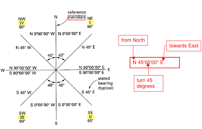 Figure 12: Bearing Angles
- The reference meridian can be of three types:
- True - parallel to line drawn from north pole to south pole. Same everywhere on Earth at any point in time
- Magnetic - taken by compass. Not equal to true meridian! Magnetic pole is constantly changing and depends on where you are on Earth
- Grid - An imaginary grid is superimposed on to a map. Angle references this grid
- Magnetic declination is the difference between True meridian and Magnetic meridian
- Agonic line = Line where magnetic meridian = true meridian
- Isogonic line = The “topographic” line that shows the same magnetic declination is called
declination = angle from TRUE to MAG
\[TRUE = MAG + DECLINATION\]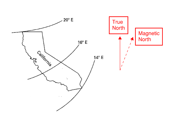 Figure 13: Isogonic Contours
4.3 Azimuth
- Azimuth is a measurement that starts North and rotates CLOCKWISE ranging from 0 to 360 degrees.
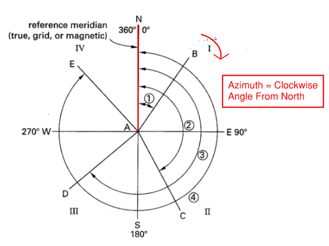 Figure 14: Azimuth
- Same as above, Azimuth can either be 1.) true, 2.) magnetic, or 3.) grid.
- A common mistake is thinking 90 degrees = 180 degrees…
4.4 Traverses
- Traversing is the task of relating points through angles and distances. There is Open Traverse and Closed Traverse
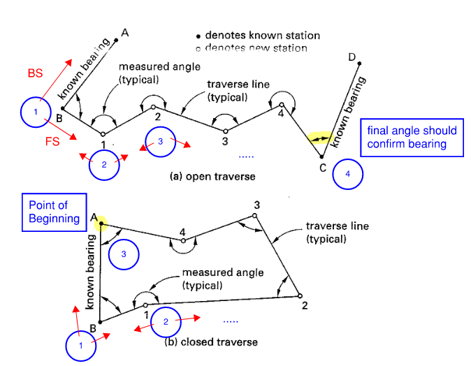 Figure 15: Open and Closed Traverse
- For closed traverse, the internal angles must add up to the following where n = number of legs (e.g. triangle = 3)
We will discuss traverses in detail in Chapter 6.
\[\sum \theta_{exterior} = 360N_{angle} - \sum \theta_{interior}\]5.0 Error Analysis and Distribution
It is impossible to measure things exactly without error. Sources of error can be systematic or random. Here is a list of potential sources:
- Procedure shortcomings
- Care exercised by surveyor
- Equipment calibration frequency
- Weather
Level of Accuracy is the measure of uncertainty regarding the survey overall. For any survey, you can exercise an extreme amount of care. In order to establish uniformity and prevent oversurveying (and reduce cost), Caltrans Survey Manual provides detailed specifications for classification of accuracy
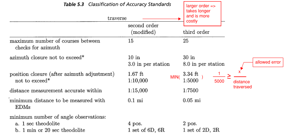 Figure 16: Caltrans Accuracy Standards
Higher order survey is more accurate, but also take longer and is more costly.
- Accuracy => how close your observed value is to the true value
- Precision => how close together your repeated measurements are to each other (could be precise but inaccurate)
5.1 Data and Error
The figure below shows some example angle measurements.
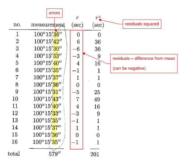 Figure 17: Error in Measurements
-
Mean of the measurements can be calculated as shown:
\[\mu = \frac{\sum X_i}{N}\]- Where \(X_i\) is the sum of all measurements, N is the number of measurements
- For multiple angle measurements, simply average the seconds if degree and minute is unchanged.
- Otherwise, add degree, minute, second separately, then use calculator function to automatically aggregate them. In the example above => 1600 degrees, 240 minutes, 579 seconds, then convert => (1604,9,39)
-
Residual is the difference between each measurement and the mean (note that residual can be negative). Also sometimes referred to as deviation.
\[r = X_i - \mu\] -
Standard Deviation is a measure of dispersion of data (how flat the bell curve is). One standard deviation of the mean value contains 68.27% of the sample. Variance is defined as \(\sigma^2\)
\[\sigma = \pm \sqrt{\frac{\sum r^2}{N-1}}\]
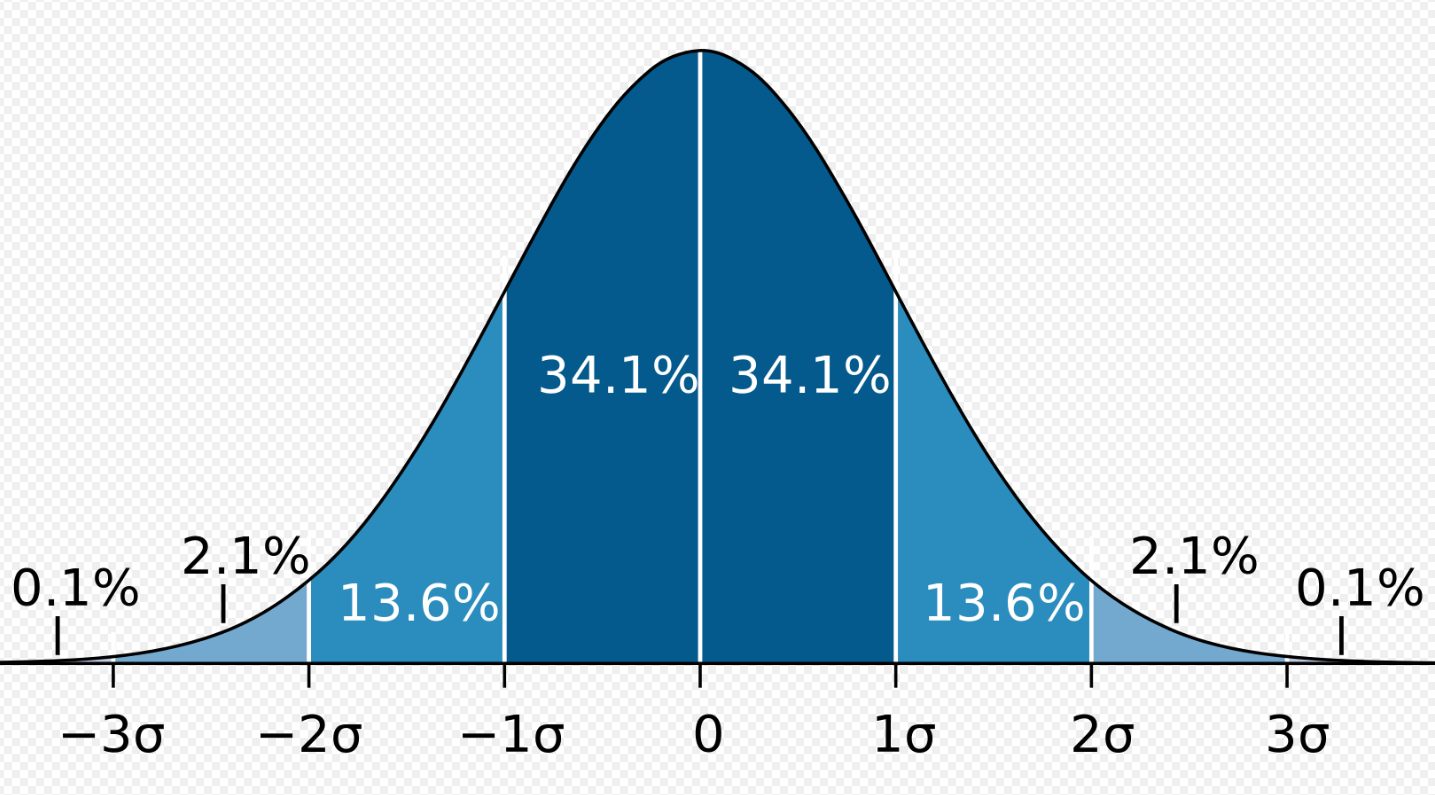 Figure 18: Standard Deviation
-
Standard Error of the Mean is a measure of uncertainty regarding the mean and is calculated as a function of sample size and standard deviation. If our sample is the entire population, then the standard error of the mean is zero. Smaller sample size = more uncertainty, and vice versa.
\[\sigma_m = \pm \frac{\sigma}{\sqrt{N}}\]- In the example above, we had 16 measurements and the standard error of the mean is \(\pm 1\)”, which means our average value is about 1” plus or minus from the true value. If we made 1,000,000 measurements, we would get even closer to the true value
- This is what we usually referred to when we say we are uncertain to \(\pm x\)”
5.2 Groups of Measurements
Say you have a traverse with 4 courses. Each course you took 20 measurements. In this case:
- Number of groups = 4
- N of each group = 20
The total standard deviation of the entire group is calculated as:
\[\sigma_{sum} = \pm \sqrt{\sigma_1^2 + \sigma_2^2 + \sigma_3^2 + ... + \sigma_n^2}\]For example,
\[(10 \pm 0.05) + (15 \pm 0.01) = (25 \pm \sqrt{0.01^2 + 0.05^2})\]Example 1: A party chief and his chainman can read the tape end to \(\pm 0.01\) ft with a 100 ft tape. What is the uncertainty in a 1000 ft distance measurement? Note that each tape reading occurs “twice” (one at each end)
- Note that if \(n = 1\), then \(\sigma_m = \sigma = \pm 0.01\) ft
- But since the tape reading rely on two readings, the standard deviation needs to be modified slightly: \(\sigma_m = \pm 0.01\) ft and \(n = 2\), thus \(\sigma = \sigma_m \sqrt{n} = \pm 0.014\) ft
- For a series of 10 grouped measurements: \(\sigma_{sum} = \sqrt{0.014^2 \times 10} = \pm 0.04\) ft
Example 2: Three distance segments measured had uncertainty of +-0.05 ft. Another four distance segments measured had uncertainty of +- 0.1 ft. What is the total uncertainty in the seven segments?
\[\sigma_{sum} = \sqrt{ 0.05^2 \times 3 + 0.1^2 \times 4 } = \pm 0.218 ft\]Example 3: Error of computing an area. Let L and W be the length of width of a rectangle
\[error = \pm \sqrt{L^2 e_L^2 + W^2 e_W^2}\]6.0 Traverses
6.1 Conceptual Stuff
Traverse is simply measuring distance and angles. Here are some definitions that you should know:
- bearings - horizontal angle measured
- headings - horizontal distance measured
- Course or Leg - course or leg of a traverse is described by a distance and an angle. The angle may be provided in bearing or azimuth
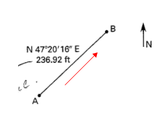 Figure 19: Course or Leg
- Departure - change in X-direction
- Latitude - change in Y-direction
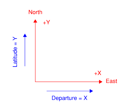 Figure 20: Departure and Latitude
Here is a tip for quicker angle calculation. Think of cosine as projection. Since bearing is always provided with respect to vertical axis (N-S), the following always holds true:
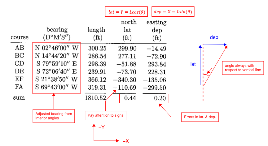
\[latitude = \Delta Y = L \cos(\alpha)\] \[departure = \Delta X = L \sin(\alpha)\]Also make sure you assign the correct sign(+,-). If using azimuth, the sign is automatically taken care of.
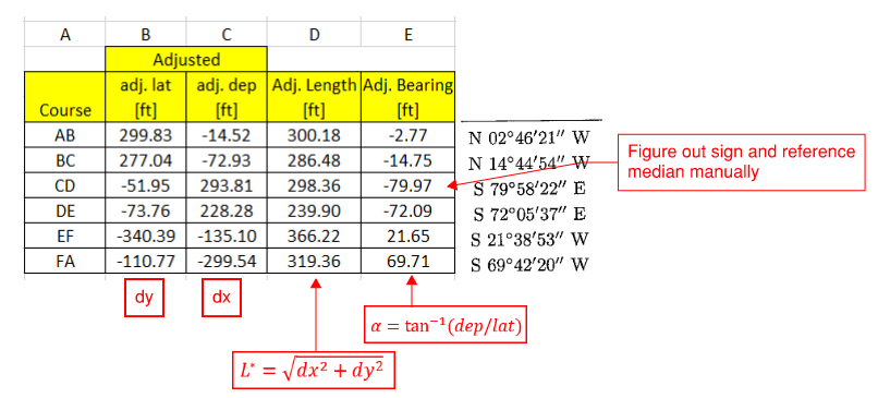
Given departure and latitude, the overall course length can be calculated using Pythagorean Theorem (easiest), or any trig ratios (sin/cos/tan). This is called inversing the course.
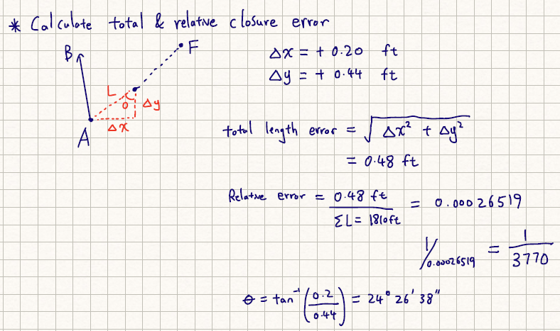
\[L = \sqrt{\Delta X^2 + \Delta Y^2}\]6.2 Closed Traverse
Closed traverse involves several courses that ultimately return to the starting point. The algebraic sum of departure and latitude should be zero. But this will never be the case no matter how careful the surveys performed. Error correction will need to be performed.
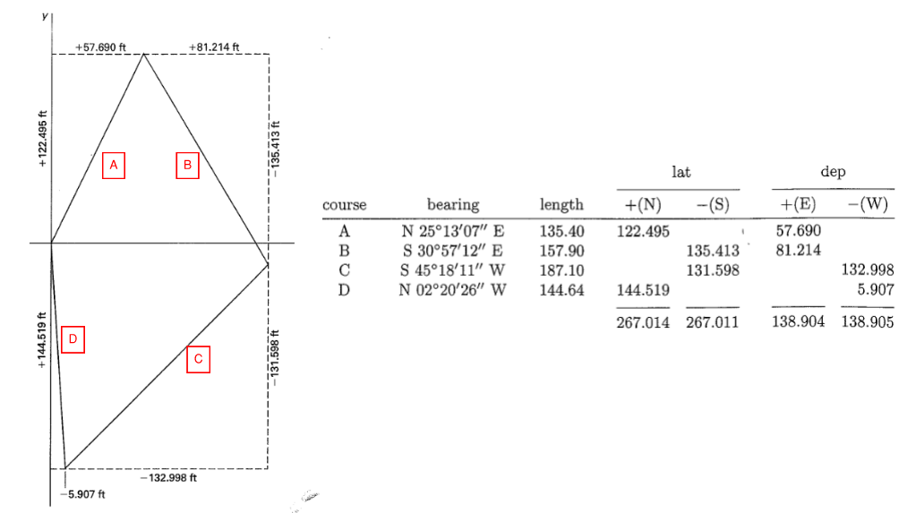 Figure 21: Closed Traverse Notes Example
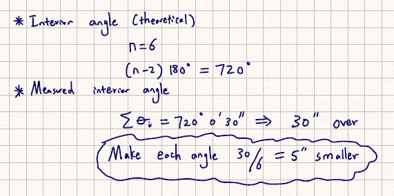
The procedure for balancing a closed traverse is lengthy and involves 1.) first balancing bearing angle with interior angle 2.) then balancing departure and latitude, 3.) then balancing bearing angle again along with length based on adjusted dep. and lat. The procedure is as follows:
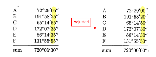
- First balance the interior angles \((n-2)\times 180^o\)
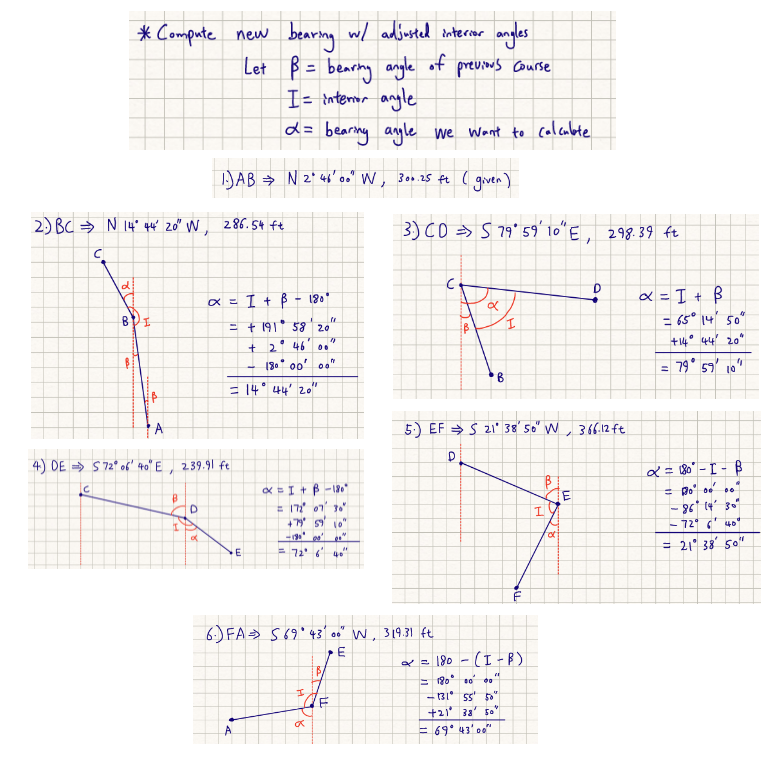
- Revise bearing of each course based on adjusted interior angle (adjusted bearing)
- Compute departure and latitude based on adjusted bearing (uncorrected dep. & lat. based on adjusted bearing in the previous step)
- Compute error in departure (dx) and latitude (dy)
- Adjust departure and latitude using compass rule (adjusted dept. & lat.)
- Finally recalculate length and bearing angle with the adjusted departure and latitude (length and bearing recalculated)
There are three methods for error adjustment of closed traverses:
-
transit rule - adjustment in proportion to latitude. Use when angular measurement is considered more reliable
\[C_x = \frac{lat_i}{\sum |lat_i|} \times dx\] \[C_y = \frac{lat_i}{\sum |lat_i|} \times dy\] -
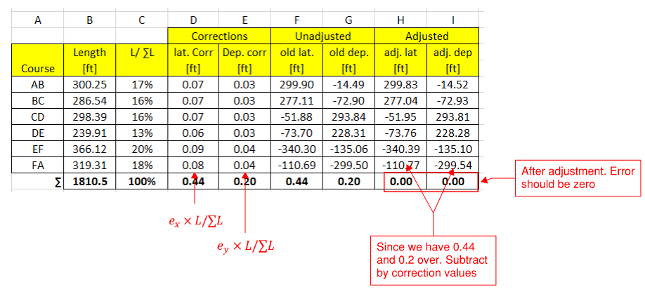
compass rule - adjustment in proportion to leg distance. Use when angular and linear measurements have equal reliability. Regarded as superior to transit rule.
\[C_x = \frac{l}{L} \times dx\] \[C_y = \frac{l}{L} \times ly\]where:
- “l” here is the length of a single course. NOT cumulative as was the case for open-traverse correction
- “L” is the total length of traverse (perimeter)
- “dx” and “dy” are the errors in dep. and lat.
-
method of least square - can be used in all cases and utilizes curve fitting. Mostly done through computer software. Too tedious by hand
To illustrate this process, we will do an example. Balance the following closed traverse with compass rule:
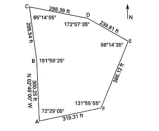 Figure 22: Example Problem for Closed Traverse
-
Balancing interior angle
-
Adjust interior angle
-
Compute new bearing based on adjusted interior angle
-
Compute latitude and longitude based on bearing in step 3
-
Calculate total and relative closure error
-
Use Compass Rule to get adjusted lat. & dep. (Measured - True). Negative means too short.
-
Recalculate final length and bearing angle
6.3 Open Traverse
Open traverse does not start and end at the same location. It can be balanced only if the start and end points are known.
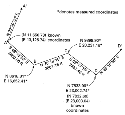 Figure 23: Open Traverse
The adjustment procedure is as noted:
- Calculate the difference between calculated and known coordinates (dx, dy)
-
Compute total and relative error of closure
\[d_{total} = \sqrt{dx^2 + dy^2}\] \[d_{relative} = \frac{d_{total}}{L}\] -
Correction to departure is calculated as:
\[C_x = \frac{l}{L} dx\] -
Correction to latitude is calculated as:
\[C_y = \frac{l}{L} dy\]where:
“l” is the cumulative distance from the beginning point
“L” is the total traverse distance
- Correct the northings (Y-axis) based on the above equations
- Correct the eastings (X-axis) based on the above equations
- Compute the adjusted rectangular coordinates (pay attention to signs)
- Adjust the length and bearing of each course accordingly based on the adjusted grid
6.4 Rectangular Coordinates
Often, a coordinate (x,y) is assigned to the starting point. From the departure and latitude measurements, the coordinate of every other point can be determined. The process is simple but pay attention to signs! And:
\[departure = \Delta X\] \[latitude = \Delta Y\]6.5 Enclosed Area - DMD Method
Closed traverses must be balanced before calculating its area. The most common method is called Double Meridian Distance (DMD) method. Area is calculated by summing the product of latitude and DMD for each course.
\[A = \frac{\sum lat_i \times DMD_i}{2}\]- Reference meridian (a vertical line) is drawn at the most westerly point
- Meridian Distance (MD) is the distance between this vertical line, to the mid point of any course. Refer to the figure below
- Make sure to calculate DMD for each course separately to avoid having error propagate through your calculation
- Divide by 43560 to convert from ft2 to acres
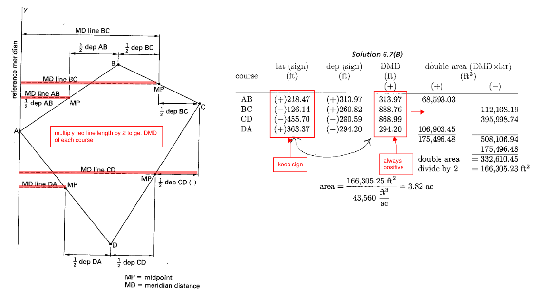 Figure 24: DMD Method for Calculating Enclosed Area
6.6 Enclosed Area - Criss Cross Method
Another more numerically convenient way of calculating enclosed area is the Criss Cross Method. But we need to get the grid (x,y) coordinates first before we can use this method. An example of this method is shown below.
 Figure 25: Criss Cross Method for Calculating Enclosed Area
A couple of COMMON ERRORS when applying criss-cross method
- Repeat the first point!
- Notice that “y” is on the first column
- Remember to divide by 2
- Translate all points to the top right quadrant before computing
7.0 Topography
7.1 Conceptual Stuff
- Topography - process of mapping elevations and physical features of a site in plan view. Also sometimes include annotations of natural or man-made features
- Horizontal Control - known point of line such as property line, centerline of highway, streets, etc.
- Vertical Control - known elevation/datum. Usually use the National Vertical Geodetic Datum (NVGD 1929) or the North American Vertical Datum of 1988 (NAVD 88)
- Four methods:
- Cross-section method - great for roads
- Grid method - great for contour
- Radial method - great for single point of interest
- Radiation method - fastest
There is also photogrammetry which involve aerial photos. We will discuss this further in future chapters.
7.2 Cross-Section Method
- Mostly used for roads. Cross sections for elevations are taken at right angles (offset lines). Refer to the figure below.
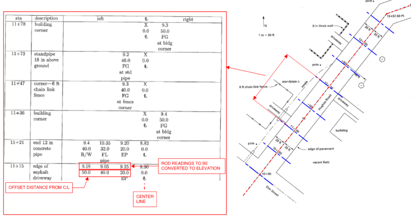 Figure 26: Cross Section Method
- Baseline (horizontal control) is usually the proposed centerline of a road or highway. Features and other point of interest are fully described in terms of:
- vertical (its elevation)
- horizontal (station along baseline + offset distance to feature)
7.3 Grid Method
- Method involves superimposing a grid onto an area of interest (divided into series of square regions). Refer to the figure below.
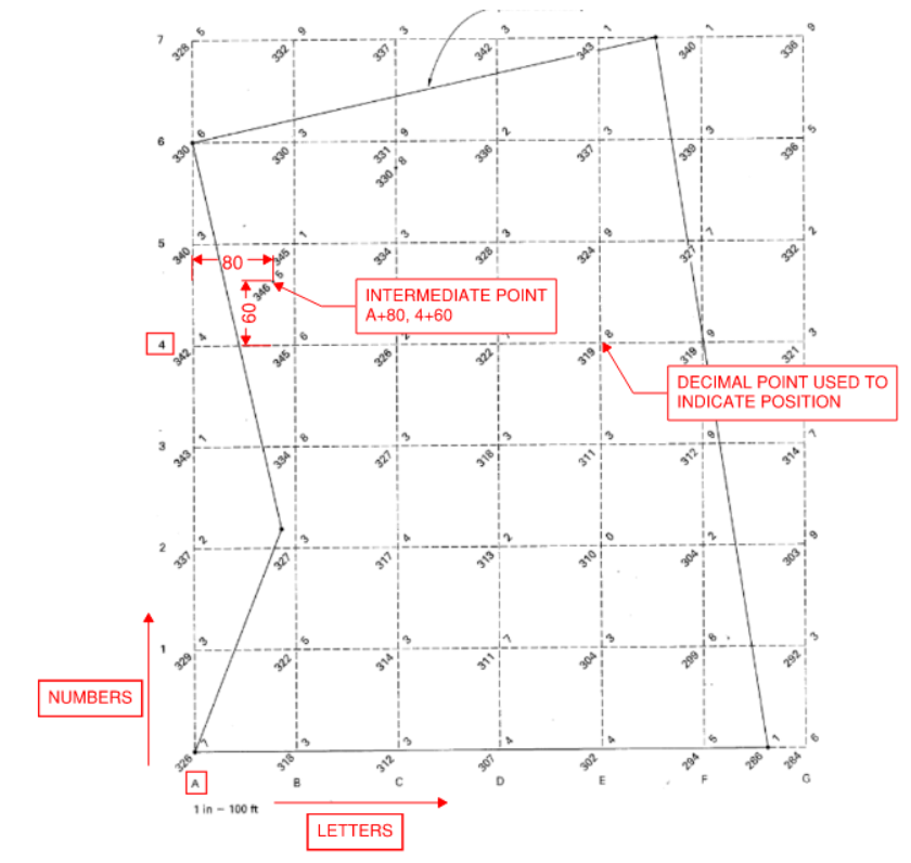 Figure 27: Grid Method
- Determine elevation at every intersection point. Then enter the data into a software to generate contour plot
7.4 Radial Topographic Survey
- Method commonly used to map a special point of interest. Start at a known point/elevation. Use stadia or total station an traverse to point of interest.
7.5 Reading Contour Maps
- Contour maps show lines of equal elevation
- The direction of a contour at any point is at right angles to the direction of steepest slope
- Contour lines cannot cross each other
- Slope (or gradient) can be determined by dividing elevation change by horizontal distance:
- Profile is kind of like a section cut on the contour:
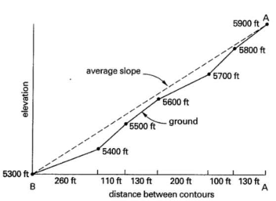 Figure 28: Contour Profile
The figure below shows some of the common features of contour plot that you should recognize.
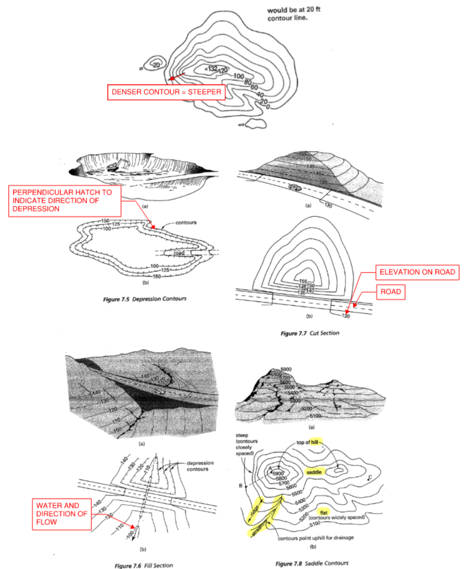 Figure 29: Common Contour Features
8.0 Route Surveying
8.1 Conceptual Stuff
Route surveying usually involve two types of curves:
- Horizontal curves - curves in direction (e.g. ramps of highway or bridge)
- mathematically circular
- straight portions are called tangents
- Vertical curves - changes in elevation and slope
- mathematically equal-tangent-parabolic
- curve can be sag or crest

8.2 Horizontal Curves
Equation and elements of a circular horizontal curve is shown below:
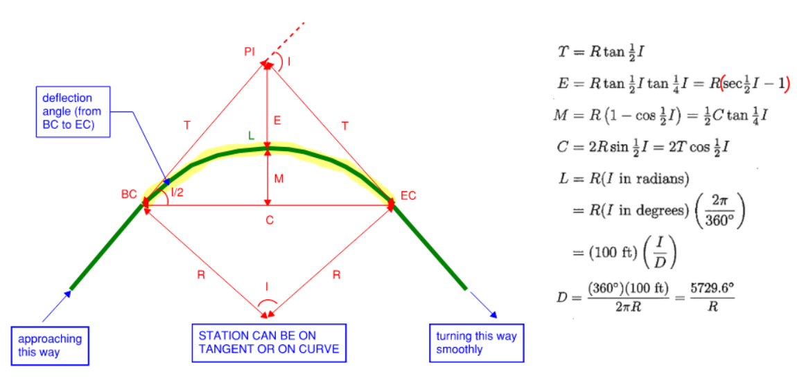 Figure 30: Horizontal Curve
Some other equations:
- Area enclosed within “E” region shaped like a boomerang:
- Area of polygon inscribed by R and T:
- Area of curve sector:
- Finding station of EC from PI
Note we CANNOT do sta_PI + T because length of curve is not equal to 2T!
Notations:
- C = long chord length from start to finish (straight line)
- D = degree of curvature
- E = external distance
- I (or \(\Delta\)) = interior angle, intersection angle
- I/2 = full deflection angle for the long chord
- L = length of curve
- M = middle ordinate
- PC (or TC or BC) = START. point of curvature, tangent-to-curve, beginning-of-curve
- PI (or V) = point of intersection, vertex, intersection of tangents
- POC = any point on the curve
- PT (or CT or EC) = END. point of tangency, curve-to-tangent, end of curve
- R = radius of curve
- T = tangent distance. Semi-tangent. (see diagram)
Degree of Curvature
Degree of curvature (D) is a measure of rate of change of rotation. Usually it is stated mathematically as 1 over radius of curvature:
\[\kappa = \frac{1}{\rho}\]However, we like to express curvature as “degree per station” rather than per feet. Note how there is a direct relationship between D and R (knowing one automatically reveals the other)
\[D = \kappa = \frac{100 ft}{R} [radian]\] \[D = \frac{5729.6^o}{R} [degrees]\]For railroad projects with very large radius, the chord basis may be preferred:
\[sin(\frac{D}{2}) = \frac{50 ft}{R}\]Deflection Angle
In the process of laying out a road, construction stakes must be installed at BC and EC and along the road at full stations (sometimes half if turn is sharp).
Deflection angle is defined as the angle between the tangent and a chord (see figure below for clarification)
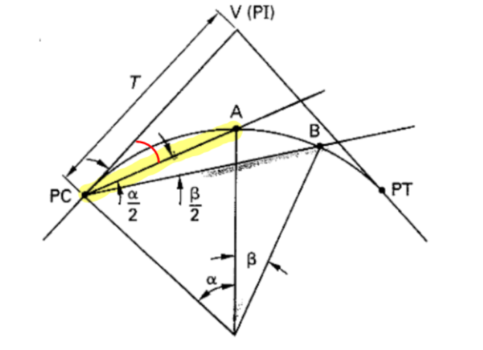 Figure 31: Deflection Angle
- highlighted area can be calculated as area of sector minus the triangle
- \(\alpha\) in the figure above is I, but could actually be any point on the curve
- \(\beta\) is another useful geometric property to keep in mind
In essence, what we want is for any two points on a curve, how much should we turn? And what is the arc length between them?
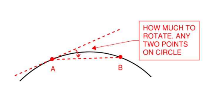 Figure 32: Deflection Angle Between Any Two Points
The deflection angle (\(\delta\)) between point A and B is simply the arc length divided by the radius divide by 2:
\[\alpha = \frac{(AB)_{arc}}{R} [radians]\] \[\alpha = \frac{(AB)_{arc}}{R} \times \frac{180}{\pi} [degrees]\] \[\delta = \alpha /2\]The chord length between point A and B:
\[(AB)_{chord} = 2 R sin(\delta)\]The deflection angle per full station can be calculated as:
\[\delta = \frac{1}{2} \times \frac{100 ft}{R} [radians]\] \[\delta = \frac{1}{2} \times \frac{100 ft}{R} \times \frac{180}{\pi} [degrees]\]Another useful parameter is deflection angle per foot. To get the deflection angle at any station, simply multiply this value by the distance from BC to the point under consideration:
\[\delta /ft = \frac{I/2}{L}\]From this exercise, we can sight the entire curve at BC by specifying how much to turn, and the corresponding chord distance.
Tangent Offset
Tangent offset can be calculated via the following
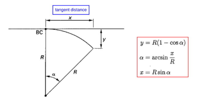 Figure 33: Tangent Offsets
8.3 Vertical Curves
Vertical curves are used to transition between grades. They can be symmetric or asymmetric. However, point V is always equidistant to PVC and PVT
 Figure 34: Vertical Curves
Notations:
- BVC, PVC = beginning of curve
- EVC, PVT = end of curve
- g1 = starting grade (%)
- g2 = ending grade (%)
- L = HORIZONTAL length of curve
- M = middle ordinate (usually very small)
- V, PI, PVI = vertex point
Since the grade typically very small. The chord distance (BVC to V and V to EVC) is essentially equal to the length of the curve.
Elevation of every point on the curve can be defined using a parabolic equation. A parabolic curve is completely defined by two grades and a horizontal length.
NOTE: r can be negative as is the case in crest curves.
\[r = \frac{g_2 - g_1}{L}\] \[y_{BVC} = y_{PVI} + g_1 (L/2)\] \[y_{elev} = (r/2)x^2 +g_1 x + y_{BVC}\] \[x_{crit} = \frac{-g1}{r}\] \[M = \frac{|g_1-g_2| L}{8}\]Units for length in stations (sta):
- \(g_1, g_2\) is in whole percents (e.g. 2, -1.5)
- \(L, x\) is in stations (e.g. 5.0, 6.5, 10.0)
- \(y_{BVC}\) elevation is in feet
Units for length in feet (ft):
- \(g_1, g_2\) is in decimals (e.g. 0.02, -0.015)
- \(L, x\) is in ft (e.g. 500, 650, 1000)
- \(y_{BVC}\) elevation is in feet
If elevation at PVI is given, can simply use the straight grade lines to back-calculate elevation at BVC or EVC. Length to BVC or EVC is usually taken to be equidistant. Remember station is in horizontal distance.
\[y_{BVC} = y_{PVI} + g_1 L_1\]If the curve is not symmetric, you may need to solve the length of curve on either side of PVI first:
 Figure 35: Solving for BVC and EVC Location Given Different Slopes
A spreadsheet table could be set up to organize calculation:
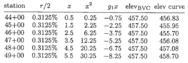 Figure 36: Vertical Curve Elevation Calculation Table
Sample calculation for sta unit:
\[456.08 = (0.625/2)(3.5)^2 - (1.5)(3.5) + 457.5\]Sample calculation for feet unit:
\[456.08 = (0.0000625/2)(350)^2 - (0.015)(350) + 457.5\]8.4 Other Types of Curves
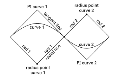
- Compound Horizontal Curve - two horizontal curve of different radius that lie on the same tangent. Analyze as two separate curves. All previous equations apply
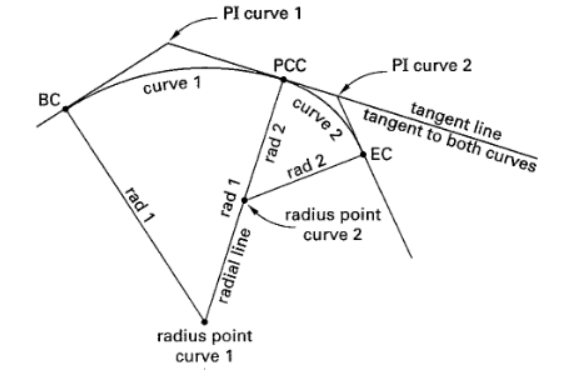
- Reverse Horizontal Curve - same as above but the second curve flips curvature
- Spiral Horizontal Curve - Used to produce gradual transition from tangent to circular
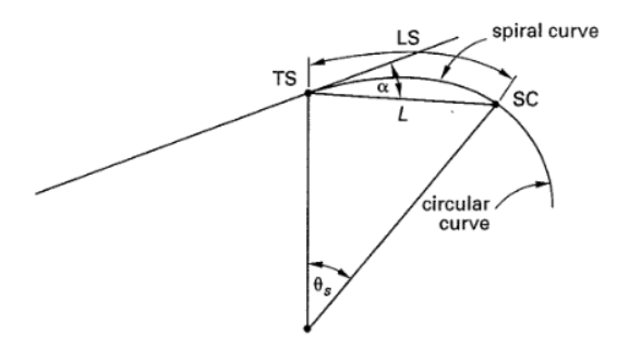
- TS = tangent to spiral
- LS = length of spiral
- SC = spiral to circle
- \(\theta_s\) = interior angle of spiral
- D = curvature of circle
- Length of spiral recommended to be a function of approach speed of vehicles. V is in mph, R is in feet
- LS can also be calculated as:
- Deflection angle for setting out the spiral can be calculated as:
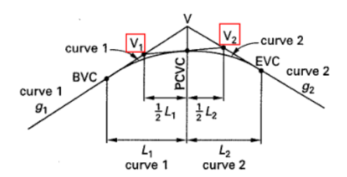
- Asymmetrical Vertical Curve - tangents are not equal. Analyze as two separate curves joined at the point of compound vertical curve (PCVC). Refer to page 67 of Cuomo text for more information and equations.
8.5 Estimating Earth Work
There are two common methods for estimating amount of soil to be cut or filled between stations. Remember to divide by 27 to convert to cubic yards.
\[VOLUME => \frac{1 \; yd^3}{27 \; ft^3}\] \[AREA => \frac{1 yd^2}{9 ft^2}\]Average End Method
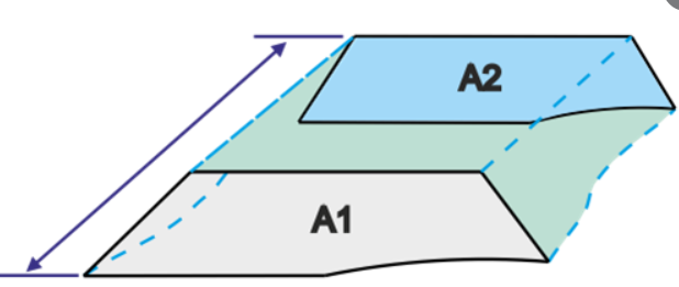 Figure 37: Earthwork Calculation Cross Section Area
Conservative and quick method. Usually over-estimates the soil. Essentially average the two end areas multiply by length.
\[V = \frac{A_1 + A_2}{2} \times L \; [ft^3]\]In some cases, one of the end area could be 0 which results in a pyramid rather than a prism. Use this formula instead if that is the case:
\[V = \frac{A_{base}}{3} \times L \; [ft^3]\]Prismoidal Method
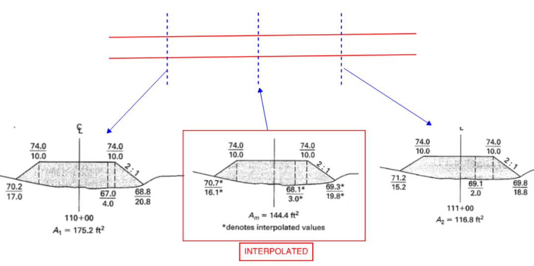 Figure 38: Prismoidal Method
If the ground is very irregular, or the two end areas differ drastically, the prismoidal method could be better. Essentially we interpolate a cross-section between the two ends, and a weighted average is taken. Usually produces smaller volume than average-end method.
\[V = \frac{A_1 + 4A_m + A_2}{6} \times L \; [ft^3]\]General Formula for Highway Sections

The formula above is a simplified express from the following sequence:

Effect of Shrinkage
Sometimes effect of shrinkage and swell are considered in earthwork calculations.
- (1) Bank volume = natural state
- (2) Loose volume = volume when its in the trucks, disturbed and loose
- (3) Compacted volume = volume after compaction
- Swell = (2) / (1)
- Shrinkage = (3) / (1)
Mass Diagram
Mass diagrams are often produced to best plan hauling schedules.
The grade is represented as y(x), then the mass ordinate is the integration of y(x) that shows the cumulative volume. Let the width of a profile slice be b(x):
\[V = \int_{0}^{x} b(x) y(x) dx\]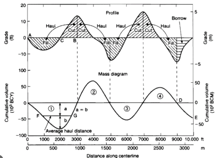
9.0 Construction Staking
9.1 Stake and Laths
Stakes are placed by surveyor to guide contractors in laying out the construction project.
- A topographic survey must be performed prior to staking to establish horizontal and vertical datum
- In some cases, construction staking is critically important:
- Determining earthwork quantities. Need to ensure correct vertical measurement. Very expensive mistake…
- Determining elevation for drainage devices. Mistake in staking for concrete gutter (which only has 0.25% slope) could lead to inadequate drainage
Stakes (Ginneys) are usually small 1” by 2” spikes that is drilled into the ground.
Laths (Ground stakes) are the actual poles containing information. They are about 2” by 36” in dimension.
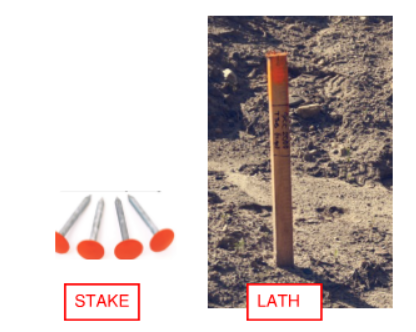 Figure 39: Stake and Lath
Fundamentally, the goal of construction staking is simple. Present information on a stick in the most concise and terse way possible. You should be familiar with some short-hands but in general just know there are often deviations from common practice and this isn’t exactly a science.
Some possible information shown on a stake (not exhaustive at all)
- Station or line - horizontal location of the stake (e.g. 25+00, property line)
- Offset - some stakes must be offset from the actual location because it would otherwise impede construction (e.g. 3.00 to curb face, 10 to cl pipe)
- Cut (C) or fill (F) - indicates whether to excavate or fill or keep as is (grade) (e.g. C 1.75 to top of curb, F 1.96 to top of wall)
- Elevation - Elevation at top of stake is marked on the lath (e.g. elev = 123.76)
9.2 Types of Stakes
Slope Stakes
- Slope stakes - used to indicate earthwork involved in creating a nice slope. Here are some example interpretations:
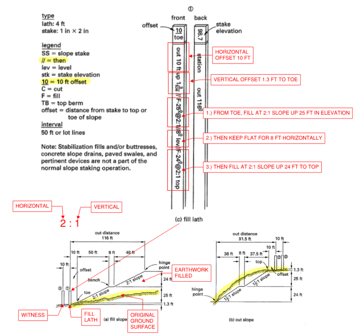 Figure 40: Reading Slope Stakes
Some definitions:
- 2:1 => 2 Horizontal : 1 Vertical
- 1/2 => 1 Vertical / 2 Horizontal
- 40% => 40 Vertical / 100 Horizontal
- Toe - bottom of slope
- Top - top of slope
- Catch Point - where slope intersect with existing ground
- Hinge Point - Upper or lower limit of the slope, usually shoulder of a road (see next figure for illustration)
- Slope Ratio - HORIZONTAL:VERTICAL
- RPSS - reference point slope stake. The offset stake
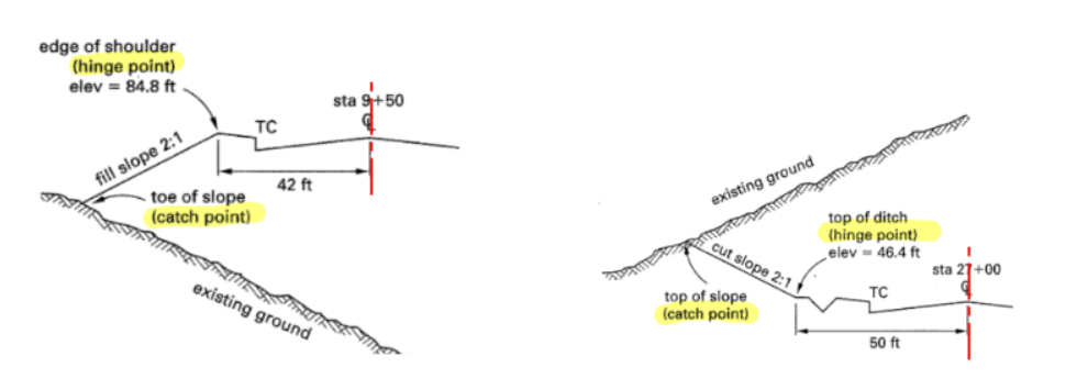 Figure 41: Some Slope Definitions
Other Types of Stakes
- Contour stakes - Used to demarcate contour lines
- Rough grade stakes - Used to control dirt grade. Not very important and is only good to nearest 0.10 ft
- Blue tops - Stakes set at a predetermined elevation. Also called “finished grade stakes”
- Building layout stakes - Offset stakes used to demarcate building footprint
- Sewer or storm drain stakes - Offset stake to demarcate sewer or storm drain lines. Usually offset by about 10 ft. Otherwise could be damaged or moved during construction
- Wall stakes - Offset stake used to demarcate retaining wall
- Curb stakes - Offset stake for curbs. Usually smaller offset (3 ft) and placed fairly close to each other (25 ft maybe closer for tighter bends). They are a drainage device so care must be taken
- Catch basin (manhole) stakes - Offset stakes. Again must take extreme care because it is a drainage device and portions of it is cast monolithically with the curb
10.0 Photogrammetry
10.1 Aerial Photogrammetry
Aerial photogrammetry involves taking measurements of site using photos taken on an airplane. Result is a topographic map with contours, elevations, and features.
- Quick but not as precise
- Does not work in wooded area
- Since multiple photographs must be taken, they need to be stitched together (known as a stereo photo)with a stereoplotter
- Therefore, photos must overlap a specific amount. Overlapping photographs are called models
In order have proper map scale. A series of control network should be established on the ground.
- AERIAL PHOTOGRAMMETRY: Minimum of (3) vertical control not in a straight line, and (2) horizontal control in overlap. Suggest using (5) each for redundancy
- GPS control survey: 3H minimum spread out (4 for kinetic GPS), 2V minimum on opposite ends.
- Control point is known as a monument and should be large and clear. Usually a large cross painted on the ground. Length of cross hair should be at least 1/1000. So for a 1:7200 scale => 7.2 ft
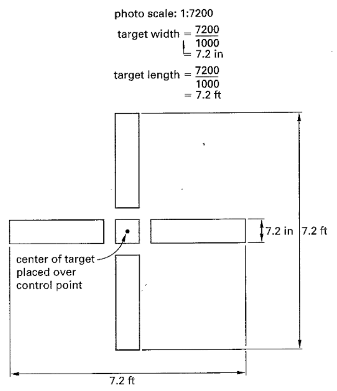 Figure 42: Control Point Cross Hair
- Alternatively, can avoid control point by using existing landmarks such as curbs, sidewalks, prominent rocks, etc. This is called post-marking.
- Contours can be generated using elevation models and interpolation
10.2 Photo Scale
Scales are expressed in two forms. Note that the two are equivalent. Convert feet to inches to go between the two.
- 1 in = 250 ft
- 1:3000
REMEMBER to multiply by 12. For example:
\[\frac{6 in}{7900 ft} = 1 in : 1317 ft = 1 in : 15800 in = 1:15800\]Scale of the photo (S) is dependent on two factors:
- Camera focal length (F)
- Flight altitude (H)
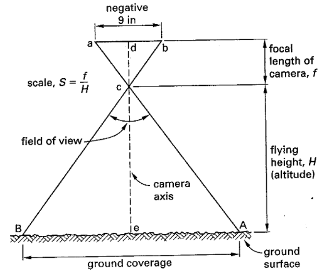 Figure 43: Photo Scale in Aerial Photogrammetry
For most project, camera focal length is fixed (typically 6 in focal length with 93 degrees field of view). Thus the variable is flight height (H).
\[H = H_{datum} - \mbox{ground elev above sea level}\] \[H = \frac{f}{S}\]Pay attention to the units!
10.3 Overlapping and Contours
To stitch two photos together, an object must show up in at least two photos (i.e. overlap). How much overlap should be provided? The common practice is to use the neat model which provides:
\[\mbox{forward overlap} = 60 \%\] \[\mbox{side overlap} = 30 \%\] \[\mbox{overlap} = \frac{\mbox{lap width}}{9 in}\]By default, photos are 9 in by 9 in
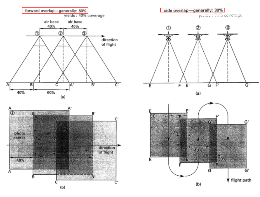 Figure 44: Model Coverage
For a 9”x9” photograph, the coverage provided by neat model is:
\[(9 in)(0.4) = 3.6 \mbox{in forward} = 4320 ft\] \[(9 in)(0.7) = 6.3 \mbox{in side} = 7560 ft\] \[coverage = 749.8 \; acre\]A intervalometer is used to automatically trigger the camera at pre-determined intervals.
At the start of most projects, the designers must provide a desired map scale (S) and contour interval (CI). Tighter CI usually means more detail is desired. The ratio between flying altitude and CI is known as C-factor
\[\mbox{C-factor} = \frac{H}{CI}\]Or CI and C-factors are given and you need to find the flying height. Then knowing the focal length, we can calculate the photo scale.
\[H = CI \times \mbox{C-factor}\] \[S = \frac{f}{H}\]There is another factor called the D-factor which is just the ratio of photo scale to map scale. Most plotters have a D factor between 5 to 8.
\[\mbox{map scale} = \frac{S}{\mbox{D-factor}}\]10.4 Flight Planning
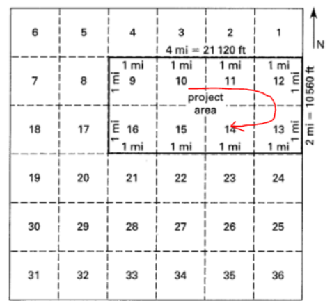 Figure 45: Flight Planning
In the project area shown above, set up required flight information given the client wants 4 ft contours. The plotter will have a C-factor of 1500. Camera will have focal length of 6 in:
-
Determine flying height (H)
\[H = CI \times \mbox{C-factor} = (4)(1500) = 6000 ft\] -
Determine photo scale (S)
\[S = \frac{f}{H} = \frac{6 in}{6000 ft} \rightarrow \mbox{1 in = 1000 ft} \rightarrow \mbox{1:12000}\] -
Determine side and forward coverage using neat model. Note that 60% overlap = 40% new information! REMEMBER (100% - overlap)
\[\mbox{forward coverage} = (9 in)(40 \%) = 3.6 \mbox{ in per photo}\] \[\mbox{forward coverage} = (3.6 in)(1000 ft/in) = 3600 ft\] \[\mbox{side coverage} = (9 in)(70 \%) = 6.3 \mbox{ in per photo}\] \[\mbox{side coverage} = (6.3 in)(1000 ft/in) = 6300 ft\] -
Determine number of flight lines => 2 lines (use smaller dimension for flight lines)
\[N_{line} = \frac{width}{coverage} = 10560/6300 = 1.7 = 2.0\] -
Determine number of models along each line => 6 models
\[N_{model} = \frac{length}{coverage} = 21120/3600 = 5.9 = 6.0\]In total, there will be 12 models required
-
Determine total number of photos required which is 1 more per line for stereoscopic coverage:
\[N_{photos} = ({N_{model}}+1)(N_{line}) = (7)(2) = 14 \mbox{photos required}\]
10.5 Height and Accuracy
Photogrammetrist will plan a control scheme, which is the ideal location to place monuments.
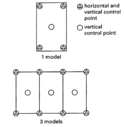 Figure 46: Placement of Control Points
The flying height we calculated before (H) is the height above mean terrain (AMT). Another useful height to calculate is the height above sea level (ASL):
\[ASL = AMT + \mbox{elevation of mean terrain from sea level}\]The following standards of accuracy must be met when using aerial photogrammetry: (note: compare scale by just using the decimal representation)
- Vertical:
- Contour - half contour interval error in not more than 10% of points tested
- Spot elevation - 90% of all spot elevation shall be accurate to within 1/4 of contour interval
- Horizontal:
- Scale larger than 1/2000 (e.g. 1/100), 1/30 of an inch error in not more than 10% of points tested
- Scale smaller than 1/2000 (e.g. 1/10000), 1/50 of an inch error in not more than 10% of points tested
- Note (1:100) > (1:12000). Calculate fraction. Don’t just look at denominator
Larger Scale = More Zoom!
- Small Scale (e.g. 1:12000)
- Map of USA
- Large Scale (e.g. 1:100)
- Map of San Francisco
Appendix: Miscellaneous Stuff
Angle Conversion
- Degree, Minute, Seconds Formula. Use built-in calculator function instead of calculating manually
- To convert the other way, for example 58.666 degrees:
- 58 degrees
- 0.666*60 = 39.96, round down to 39 minute
- (0.666 - 39/60 ) * 3600 = 57.6, round to 57 seconds
- 58 degrees, 39 minutes, 57 seconds
Unit Conversion
- 1 acre = 43560 ft^2
- 1 cubic yard = 27 ft^3
Geometry Formulas:
- Area of triangle calculation, height does not need to reside within triangle:
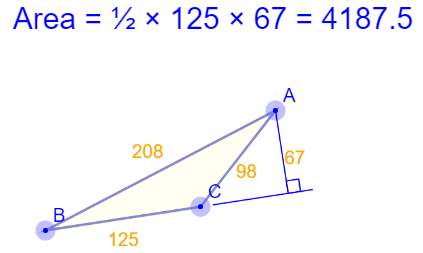
- Area of triangle given 3 sides (Heron Formula):

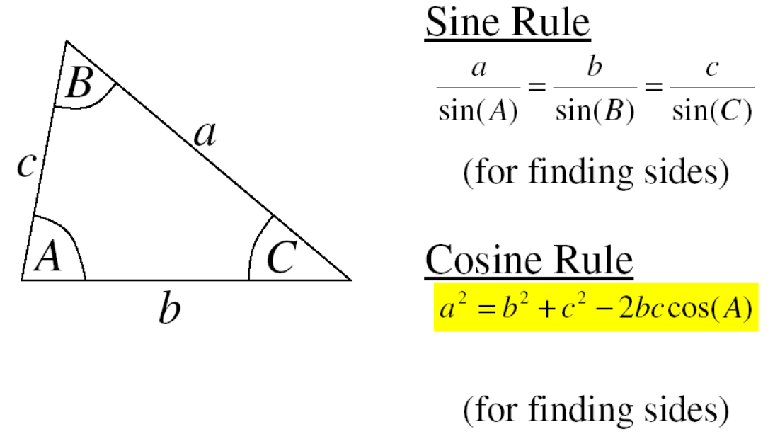
- Sine and Cosine Law:
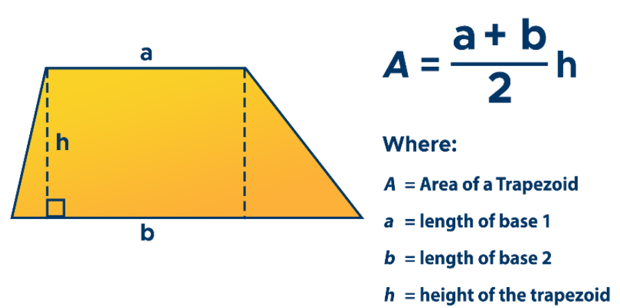
- Area of Trapezoid:
- Sector of a circle (\(\theta\) is the central angle, \(A_o\) is the area of full circle, R is radius, D is diameter)
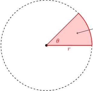
- Arc Length
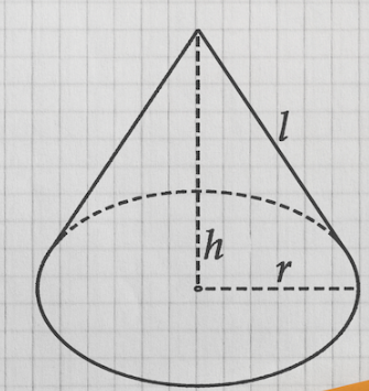
- Volume of right-circular cone
Earth Curvature and Refraction Correction
Note the negative sign for refraction correction. Also D is in feet.
\[C_{curv} = 0.0239 \frac{D}{1000}^2\] \[C_{refr} = -0.0033 \frac{D}{1000}^2\] \[C_{total} = C_{curv} + C_{refr}\]Sea Level Adjustment Factor
\[SLAF = \frac{r}{r + elev}\] \[L_{converted} = SLAF \times L_{measured}\]- r = 20,906,000 ft (radius of Earth)
- elev = elevation above sea level in ft
Things From Practice Problems:
GPS, GIS and other technologies
- Robotic total station - tracks prism automatically and can be operated by one person
- Real Time Kinematic GPS - Can be operated by one person via rover receiver. Commonly used for construction surveying. Static GPS is more accurate but too slow (about 5 min per point). Static has 0.02 ft accuracy whereas RTK has 0.1 ft accuracy.
- CORS point - permanently recording GPS station
- GPS Errors. Weather cannot impact GPS precision but atmospheric conditions does. Refraction and electromagnetic interference does! Dilution of precision occurs if satellites are too close to each other.
- GIS data type: raster = img, vector = coordinates, metadata = data about the data
- Digital orthophoto = photo image in which every pixel is in its correct map position
- Aerial Triangulation = process of determining the ground coordinates of artificial points marked on the emulsion of an aerial photo
- Planimetric Map = plan view of any drawing. Does not contain any elevation information
Standards
- Lambert Conformal Conic - projection of California state plane system
- US survey foot was introduced in the North American Datum of 1983 (NAD83) because the typical foot was not accurate enough in the NAD 1927. 3937/1200 is more accurate than 10 ft = 3.048 m. In the past, the baseline was based on Gunter Chains.
- Metes and Bounds Description = legal description involving complete perimeter of a piece of land (bearing and length)
- Legal definition of property = depends on intent of the parties to a conveyance
- NVGD 29 vertical datum (old) was adjusted to fit 26 mean sea level stations. Used prior to 1991
- NAVD 88 vertical datum (new) held one point fixed – Father Point Rimouski. Fixed to a tidal benchmark in Quebec. Supersedes NVGD 29
- NAD adjustments were purely horizontal and does not affect stationing which is relative
Underground Utilities
- Potholing is the most accurate way of finding underground utilities. Conduct field investigation first. Potholing usually occurs later on
- Underground Service Alert (Dig Alert) - a non-profit that will help identify location of underground utilities with spray paint. Not depth information though
- A pipe has three different elevations:
- Invert elevation = bottom inner
- obvert elevation = top inner
- crown elevation = top outer
Miscellaneous
- Map scale of 0.99 means 100 ft indicated is actually 100/0.99 = 101 ft
- Vertical control accuracy listed from most accurate to least:
- Global regional geodynamics
- Basic framework
- Secondary network
- General area
- Local control
- For short distances, tape is preferred over total station.
- Trigonometric leveling does not have high precision compared to BS/FS because of refraction in the atmosphere
- Invar strip - material used to achieve highest precision in leveling for tapes and rods
- Transits are old instruments used to measure horizontal distance and vertical angle, but read from a vernier scale (caliper)
- Double transit - (double centering) best method for extending a straight line with theodolite (inverting a transit)
- Two-peg test - is used to determine mislevelment of line of sight of the leveling device
- 3-Wire Leveling - very precise. Basically differential leveling w/ 3 readings for BS and FS
- Angular resolution looking through a scope can be calculated as:
Comments