EZPZ Section Analysis Development Log
2023-06-25 Update: EZPZ has been superseded! Earlier this year, I decided to rewrite and refined this project. Enough changes were made that I thought I’d just rename the project all together. Presenting fkit (fiber kit). It’s at least 10x better than EZPZ Click here for GitHub Repo
- 1.0 Inspiration
- 2.0 Fiber Analysis Algorithm For Moment Curvature Analysis
- 3.0 Object-Oriented Design
- 4.0 How Does it Work?
- 5.0 EZPZ Quick Start
- 6.0 EZPZ Full Tutorial
- 7.0 Assumption And Challenges
1.0 Inspiration
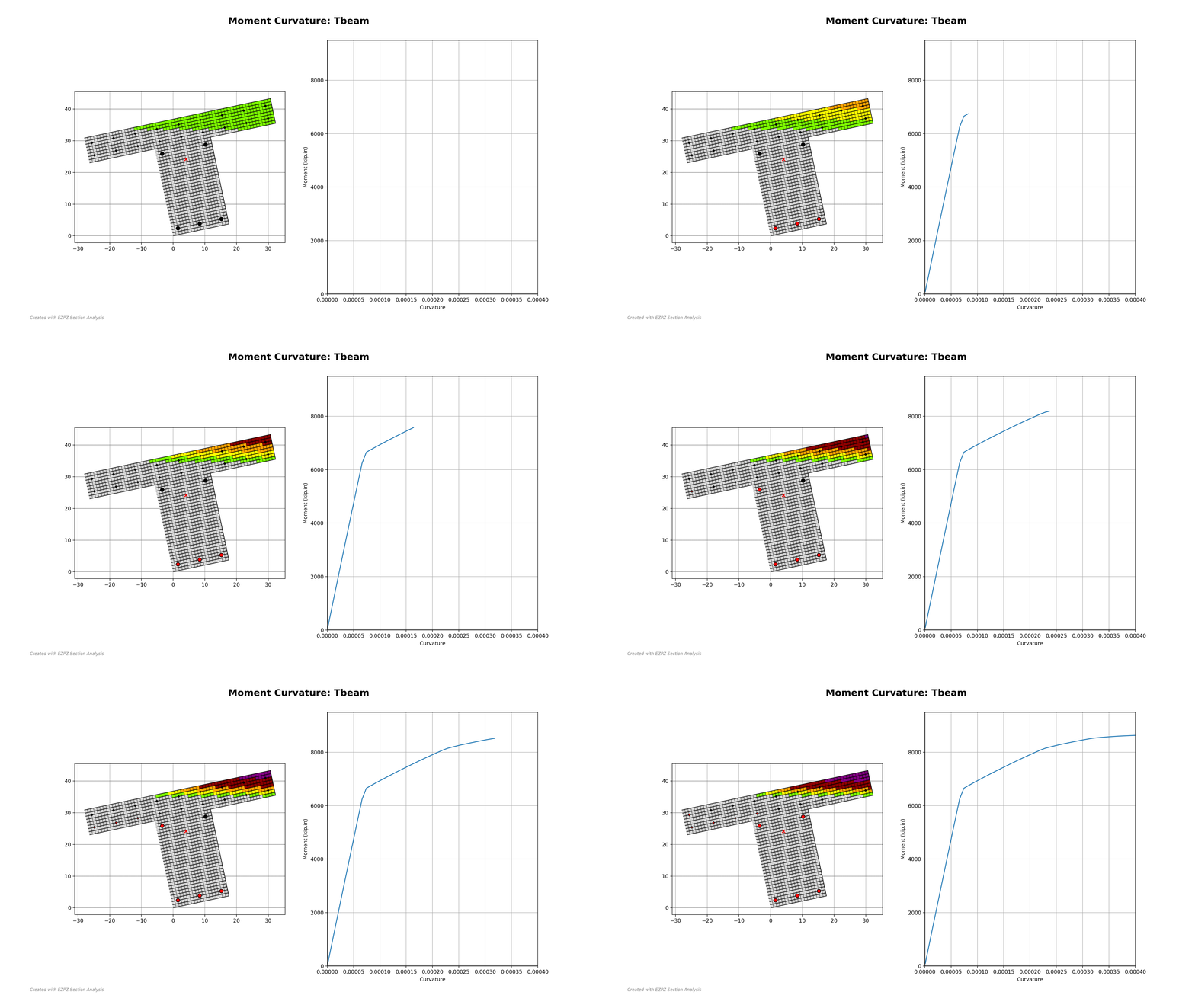 Figure 1: Animated Example Showing Capability of EZPZ
Strain compatibility analysis is a corner stone of concrete analysis/design. It is used to determine flexural capacity of many concrete elements ranging from footings, walls, columns, beams, slabs, and much more.
For most design purposes, all we care about is the ultimate moment capacity; meaning we only care about a single point on the moment curvature diagram. Furthermore, for computational simplicity, we opt to assume a rectangular compressive stress block and that all tension reinforcements (rebar) have reached their yield strength. The resulting equation is very easy to compute by hand and exceptionally convenient.
When we eventually learn about moment-curvature relationships in a more advanced concrete design class, the conventional pedagogy is to determine 4 or 5 key points along the curve. What you end up with are these very clunky k-factors and equations.
Now that we have all this compute power and scripting ease with python. I thought it would be a fun side-project to do a concrete section analysis program in python. Hopefully one that is easier to use than OpenSees, albeit less powerful. Some potential improvements to make over OpenSees:
- Avoid the need to define zero-length member… displacement control integration…etc…
- Too much boiler plate code (choosing integrator, DOF numbering, algorithm integrator, etc…)
- uni-axial material properties does not need to have full hysteresis (loading-unloading memory), just monotonic is okay
- Tedious to mesh concrete patches and rebar nodes and no built-in visualization. Need a convenient way to create sections.
OpenSees is extremely powerful and robust, but it just seems like we are swatting a fly with a sledgehammer there. Anyways let’s start coding!
2.0 Fiber Analysis Algorithm For Moment Curvature Analysis
The algorithm for moment curvature analysis is actually extremely intuitive to understand, and dare I say much simpler (once you have some programming knowledge) to apply programmatically on a computer.
Increment section curvature from \(\phi = 0\) to a desired ultimate curvature (0.0004 seems to be a good ultimate value for most sections).
- Given a curvature value (\(\phi\)), and a desired section net axial force (P)
-
Use a root-solver to determine depth of neutral axis where the integration of fiber forces sum up to P (i.e. internal forces are in equilibrium):
\[\sum P_{steel fibers} + \sum P_{concrete fibers} = P\]-
Given depth of neutral axis (c) and curvature (\(\phi\)), the fiber strain (\(\epsilon\)) can be calculated as a function of its depth from top of section
\[\epsilon = \phi c - \phi d_{fiber}\] -
Then the stress can be determined using any uniaxial material model
\[\sigma = f(\epsilon)\] -
Lastly, multiply stress by area of fiber to determine its force contribution:
\[F_{fiber} = \sigma \times A_{fiber}\]
-
-
At the neutral axis depth (c) under consideration, the section internal moment can be expressed as:
\[M = P_{steel fibers} \times e_i + \sum P_{concrete fibers} \times e_i\]where \(e_i\) is the distance between fiber centroid and section centroid.
- Now we have a single point (\(M, \phi\)). Repeat and increment curvature
3.0 Object-Oriented Design
It was clear from the outset that an object-oriented approach would be most ideal in tackling this program. The idea is to create fiber objects that store their own stress/strain state and can be easily queried with dot notation.
Three classes were defined:
- Section object
- ConcreteFiber object
- SteelFiber object
Furthermore, a set of helper functions were created to help users quickly and easily mesh typical sections. Refer to the figure below for a summary chart.
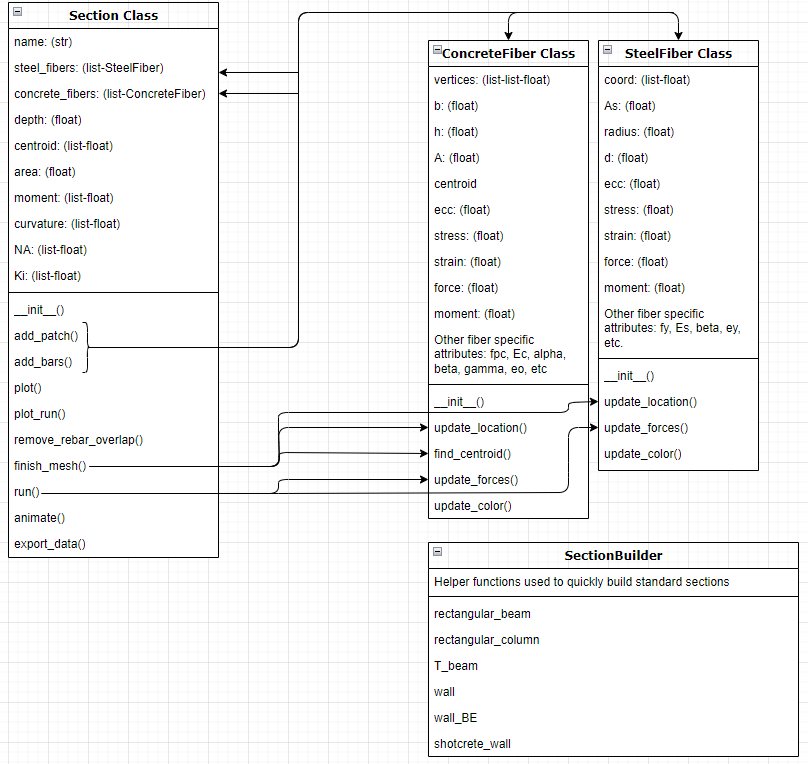 Figure 2: OOP Design Chart
4.0 How Does it Work?
A section object holds all the valuable information pertaining to a given section. It also contains two arrays holding all the concrete and steel fiber objects. By defining each fiber as an unique object, finding the stress/strain and force/moment contribution is easy using the dot notation (fiber.update_force()). The EZPZ calculation routine can be concisely summarized as follows:
- Define a section either manually or with a helper function:
- Use section.add_patch() & section.add_bar() to mesh sections manually. After the section is fully defined, run section.finish_mesh() to calculate overall centroids section geometry
- Note you can also use section.finish_mesh() to rotate the section, or specify removal of concrete_patches that overlap with steel fibers
- Alternatively, use helper functions defined in SectionBuilder.py to quickly define common sections. You can also create a function yourself if none of the current ones suit your fancy
- Use section.plot() to get a peek of the section that was just defined
- Use section.run() to conduct moment curvature analysis
- Use section.plot_run() to plot the moment-curvature diagram
- Use section.animate() to generate a series of png files at each step of the moment curvature analysis. Afterwards a gif file can be created using any third-party software such as ImageMagick
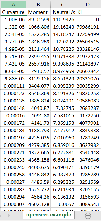
- Use section.export_data() to output a csv file containing the \((M, \phi)\) coordinates as well as neutral axis, and stiffness
In terms of dependencies and package management, a conscious effort was made to avoid unnecessary packages installation if the implementation could be done in plain python. Only well-known and well-supported packaged are used. All the imported packages are readily available and comes pre-installed with Anaconda. I will try to make a proper pip installation in the future.
- numpy - to handle arrays and matrix operations
- scipy.optimize.root - for root-finding and quickly determining depth of neutral axis
- matplotlib - for plotting results
- math - trig, rounding, sqrt, etc
- itertools - some list manipulations
- os - used to extract current working directory to output any files
5.0 EZPZ Quick Start
1. First let’s import the EZPZ package
import EZPZ
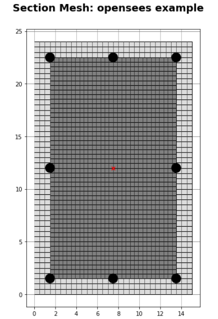
2. Let’s define the same section as the OpenSees moment curvature example
section6=EZPZ.SectionBuilder.beam_complicated(name="opensees example", b=15, h=24, cover=1.5,
                            bot=[7,3,3,21], fpc1=6, fpc2=5, fy=60,
                            alpha1=0.83, alpha2=0, beta=0, Es=29000, plot_section=True)
3. Run the analysis
section6.run(P=180, phi_max = 0.0006)
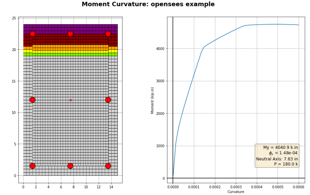
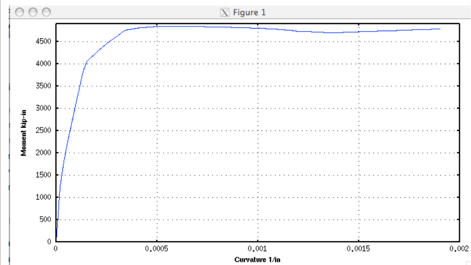
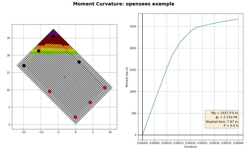
Compare with OpenSees, both have a peak moment capacity of around 4600 kip.in. Note that EZPZ’s default Hognestad concrete model differs slightly from OpenSees’ “concrete01” model.
4. Export result if desired
The plot data can be easily exported into csv format:
section6.export_data()
6.0 EZPZ Full Tutorial
1. First let’s import the EZPZ package
import EZPZ
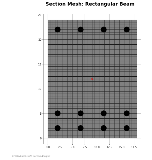
2a. Manual definition of a rectangular section
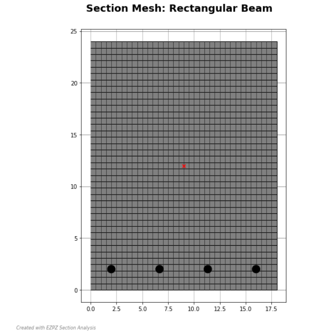
section1 = EZPZ.Section.Section("Rectangular Beam")
section1.add_bars(x0=2, y0=2, dx=14, dy=0, nx=4, ny=1, bar=6, mode="f", material="default", m_kwarg={'fy':60})
section1.add_patch(x0=0, y0=0, b=18, h=24, Nx=36, Ny=39, material="default", m_kwarg={'fpc':4})
section1.finish_mesh(plot_section=True)
Run the python help() command to see how to use section.add_bars() and section.add_patch():
help(section1.add_bars)
help(section1.add_patch)


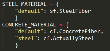
The “material” tag and the associated model parameters (m_kwarg) seems verbose but is an efficient way to specify what model the fibers should take and leaves room for future expansion. In essence, “material” is the key to a dictionary where the return value is the desired fiber class definition. Currently, there are only 3 uni-axial models defined but there are ample room for future expansion. We will discuss the current default material models in the next section.
2b. Define section using helper functions Alternatively, we can use a helper function to define the section:
section2=EZPZ.SectionBuilder.rectangular_beam(name="Rectangular Beam",
                                              b=18, h=24, cover=2, bot=[9,4,2,3],top=[9,4,1,0],
                                              fpc=4, fy=60, plot_section=True)
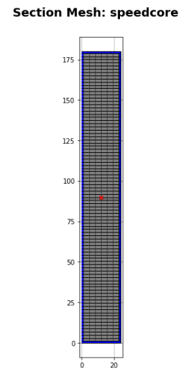
Here are some other templates currently available.
section3=EZPZ.SectionBuilder.speedcore(name="speedcore", b=24, h=180, t=1,
                                       fpc=4, fy=50, alpha=0.85, beta=0, Es=29000, plot_section=True)
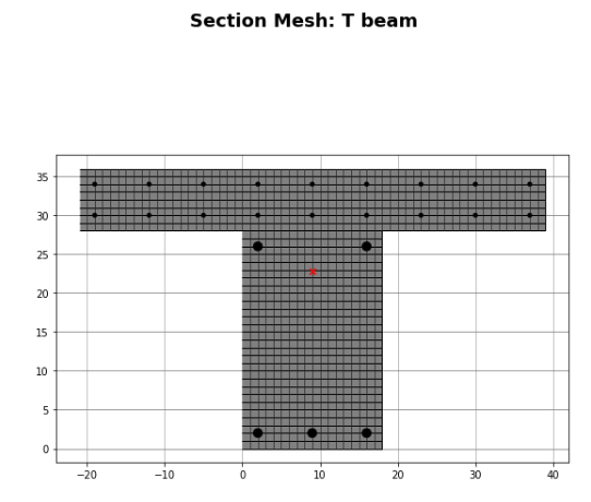
section4 = EZPZ.SectionBuilder.T_beam(name="T beam", bw=18, bf=60, h=36, tf=8, cover=2,
                                      bot=[9,3,1,0], fpc=4, fy=60, top=[9,2,1,0], slab=[4,9,2,4], plot_section=True)
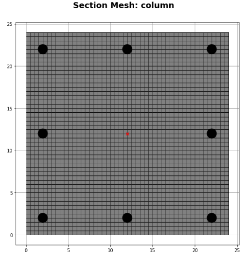
section5 = EZPZ.SectionBuilder.rectangular_column(name="column",
                                              b=24, h=24, cover=2, fpc=4, fy=60,
                                                  nx=3, ny=3, bar=9, plot_section=True)
section5=EZPZ.SectionBuilder.beam_complicated(name="opensees example", b=15, h=24, cover=1.5,
                            bot=[7,3,3,21], fpc1=6, fpc2=5, fy=60,
                            alpha1=0.83, alpha2=0, beta=0, Es=29000, plot_section=True)

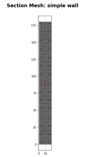
section7=EZPZ.SectionBuilder.wall(name="simple wall",b=18,h=180,cover=2,bar=7, spacing=12,
                                  fpc=5, fy=60, plot_section=True)
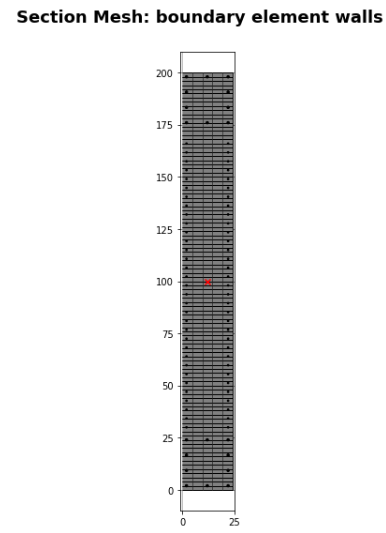
section8=EZPZ.SectionBuilder.wall_BE(name="boundary element walls",b=24,h=200,cover=2,
                                     web_bar=6, spacing=6, BE_bar=[9,3,4],L_BE=24,
                                      fpc=5, fy=60, plot_section=True)
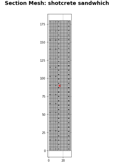
section9 = EZPZ.SectionBuilder.shotcrete_wall(name="shotcrete sandwhich",b=[12,18],h=[180,180],cover=[2,2],
                                       bar=[4,7], spacing=[12,6],
                                      fpc=[3,5], fy=[40,60], plot_section=True)
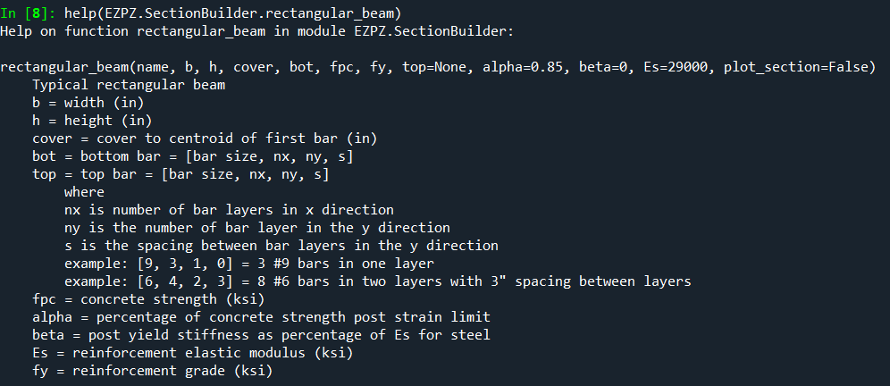
Again use the help() command to view how to use each templates:
help(EZPZ.SectionBuilder.rectangular_beam)
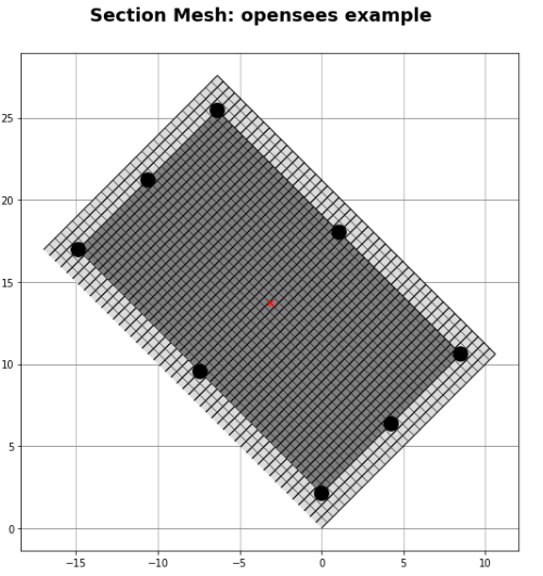
3. The defined section can be rotated if desired!
section6.finish_mesh(rotate=45)
section6.plot()
4. Run the analysis
section6.run(P=0)
5. Export data if desired
section6.export_data()

7.0 Assumption And Challenges
I’ve encountered many technical challenges and interesting puzzles throughout the development process. Nevertheless, there was never a boring moment and I appreciated all the excellent learning opportunities. Here are some of the cool things I learned.
7.1 Uniaxial Material Models
Unlike a complete hysteresis material model used by OpenSees, which keeps track of fiber state and strain history, the EZPZ material model implementation is fairly trivial. In other words, there is no distinction made between loading and unloading, a strain value will always correspond to a stress value with no regards to any other facts. (\(\sigma = f(\epsilon)\))
The default steel fiber is defined using a simple bi-linear material model, with a pre-yield stiffness and a post-yield stiffness. The post-yield stiffness is adjusted using a \(\beta\) factor which represents percentage of pre-yield stiffness retained after yielding.
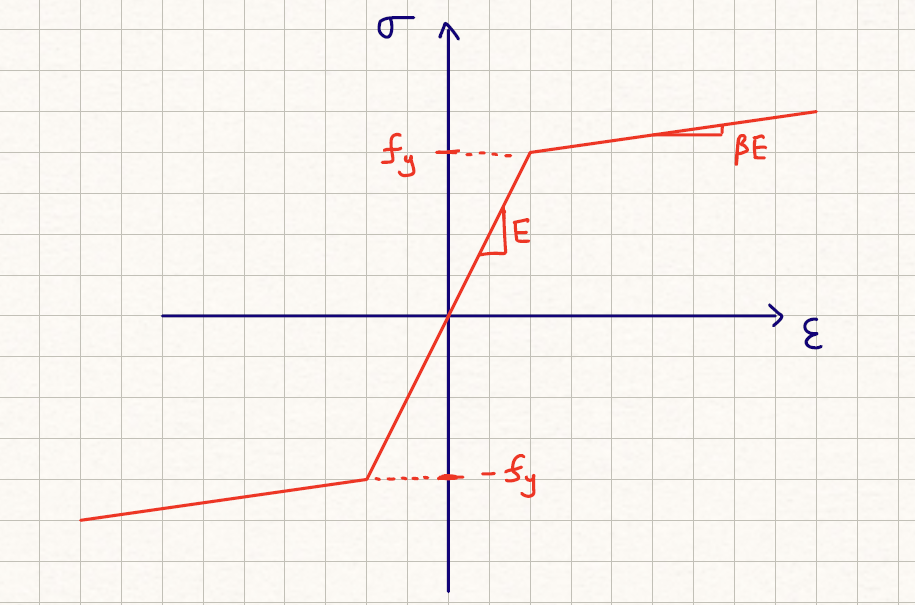
# calculate strain based on given curvature and neutral axis depth
strain = phi*c - phi*self.d
stress = self.Es * strain

# modify stress if in post-yield region
if stress < -self.fy:
    stress = -self.fy + (self.beta * self.Es*(strain - self.ey))
elif stress > self.fy:
    stress = self.fy + (self.beta * self.Es*(strain - self.ey))

# calculate force and moment contribution
force = stress * self.As
moment = force * self.ecc
As for the concrete fiber model, the default implementation is the Modified Hognestad Model as derived in Chapter 3.5 of the Macgregor and Wight concrete design textbook. The are three distinct stages:
- An initial parabolic stage up until peak strain (\(\epsilon_o\)) and peak stress of \(0.9f'_c\)
- A linear decrease stage post peak strain up until ultimate strain (\(\epsilon_u\))
- A constant stage thereafter
The residual capacity post-peak is adjusted using an \(\alpha\) factor. The recommendation is to use:
- \(\alpha = 0.85\) for confined concrete
- \(\alpha = 0.15\) for unconfined concrete
The equations are as follows:
If strain is negative, fiber is in tension; tension capacity of concrete is neglected:
\[\sigma = 0\]In the parabolic stage:
\[\epsilon_o = 1.8 (0.9f'_c) / E_c\] \[X = \epsilon / \epsilon_o\] \[\sigma = \frac{0.9f'_c}{2X-X^2}\]In the linearly descending branch:
\[\sigma = 0.9f'_c - \frac{(1-\alpha)0.9f'_c}{\epsilon_u - \epsilon_o} (\epsilon-\epsilon_o)\]Post ultimate strain:
\[\sigma = \alpha 0.9 f'_c\]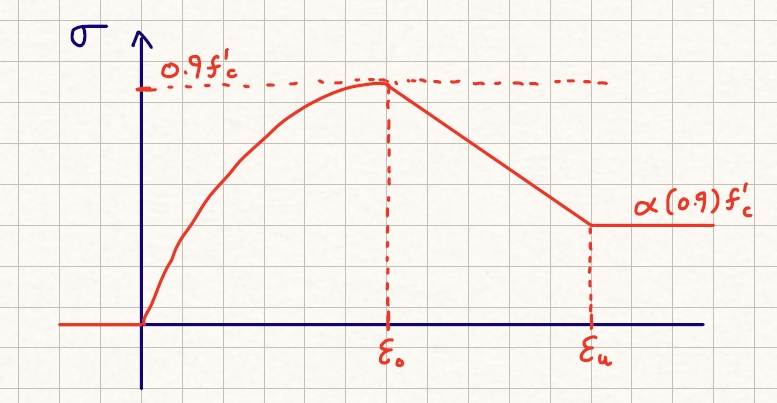
# calculate strain
eu = 0.0038
enew = phi*c - phi*self.d
eo = 1.8*0.9*self.fpc / self.Ec

# calculate stress
if enew < 0:
    stress = 0
elif enew <= eo:
    X = enew/eo
    stress = 0.9*self.fpc * (2*X-X*X)
elif enew > eo and enew < eu:
    stress = 0.9*self.fpc - ((1-alpha)*0.9*self.fpc)/(eu-eo) * (enew-eo)
else:
    stress = alpha*0.9*self.fpc

# calculate force and moment contribution
force = stress * self.A
moment = force * self.ecc
7.2 Rotating the Section By An Arbitrary Angle
Rotating the section turned out to be much easier than expected with the magic of linear algebra. I am extremely grateful to 3Blue1Brown for his excellent videos on linear algebra, which gave me the intuition for doing this.
Essentially, all fibers have a specific x,y coordinate (fiber.x, fiber.y). Rotating the section is simply a matter of applying a rotational transformation matrix to all fibers.
The pre-rotated coordinate of a fiber is given by the position vector:
\[\bar{r}=\{x,y\}\]The new coordinate after rotation is given by:
\[\bar{r'}=\{x',y'\}\]The relationship between the two is given by:
\[\bar{r'}=[T] \bar{r}\]Where the transformation matrix is defined as:
\[[T] = \begin{bmatrix} cos(\theta) & -sin(\theta)\\ sin(\theta) & cos(\theta) \end{bmatrix}\\\]Here is the implementation in python:
import numpy as np

# define transformation matrix
T = np.array([
    [math.cos(rad), -math.sin(rad)],
    [math.sin(rad), math.cos(rad)]])

# rotate section centroid
self.centroid = T @ self.centroid

# loop through all concrete and steel fibers to transformation their coordinates
for f in self.concrete_fibers:
    f.centroid = T @ f.centroid
    for i in range(len(f.vertices)):
        f.vertices[i] = T @ f.vertices[i]
for f in self.steel_fibers:
    f.coord = T @ f.coord
7.3 Meshing
Another interesting challenge came up in the form of meshing. Originally I had relied upon an external open-source library called “dmsh”. It took about 5 to 10 seconds to mesh a section with triangular elements.
However, during the development I came to a couple of realizations:
- I don’t want to rely on packages that are not readily available in Anaconda
- The meshing was kind of sluggish because it was error-checking and optimizing mesh
- I am meshing mostly rectangular sections, perhaps a mathematically rigorous mesher is unnecessary?
- Lastly, fiber analyses do not require properly connected nodes and degree of freedoms
The last point made me realize I do not need a rigorous mesher at all! It suffices to discretize a section using many rectangular blocks. They can overlap, they do not need to be connected, none of that matters! By adopting a much simpler approach, the meshing became almost instantaneous!
Here are the functions I used to mesh user-specified concrete patches. In essence, the user specify rectangular patches of concrete to form the overall section.
def add_patch(self, x0, y0, b, h, Nx, Ny, material="default", m_kwarg={'fpc':4}):
    """
    Use method to add concrete fiber to section
    x0, y0 = lower left coordinate
    b, h = width and height of patch
    Nx, Ny = used to dictate how fine of a mesh we will use
    material = tag for which material to use
    m_kwarg = dictionary of input parameters for chosen material
    """
    # generate concrete vertices coordinates
    conc_patch = []
    dx = b / Nx
    dy = h / Ny
    for i in range(Nx):
        for j in range(Ny):
            xref = x0 + i * dx
            yref = y0 + j * dy
            node1 = [xref   , yref]
            node2 = [xref+dx, yref]
            node3 = [xref+dx, yref+dy]
            node4 = [xref   , yref+dy]
            conc_patch.append([node1,node2,node3,node4])

    # generate concrete fibers
    conc_fiber=[]
    for f in conc_patch:
        m_kwarg["vertices"] = f
        conc_fiber.append(CONCRETE_MATERIAL[material](**m_kwarg))
    self.concrete_fibers += conc_fiber
The meshing for steel reinforcement is somewhat easier to implement because rebar nodes are actually 1-dimensional. One interesting functionality is specifying “perimeter” mode vs. “full” mode. The former makes a box of bars with an “empty” center(i.e. only bars on the perimeter), the latter is just a typical 2-d array.
def add_bars(self, x0, y0, dx, dy, nx, ny, bar, mode, material="default", m_kwarg={'fy':60}):
    """
    Use method to add steel fiber to section
    x0, y0 = lower left coordinate of bar array you want to generate
    dx, dy = size of rectangle bounding bar array
    nx, ny = number of bars in horizontal(x) and vertical(y) direction
    bar = bar size from 3 to 18
    mode = "f" for full array, "p" for bar only on perimeter of bounding box
    material = tag for which material to use
    m_kwarg = dictionary of input parameters for chosen material
    """
    # determine spacing
    sx = 0 if nx==1 else dx / (nx-1)
    sy = 0 if ny==1 else dy / (ny-1)

    # generate bar coordinate
    xcoord=[]
    ycoord=[]
    xcoord.append(x0)
    ycoord.append(y0)
    if sx != 0:
        for i in range(nx-1):
            xcoord.append(xcoord[-1]+sx)
    if sy !=0:
        for i in range(ny-1):
            ycoord.append(ycoord[-1]+sy)
    reinf = list(itertools.product(xcoord,ycoord))

    # remove middle bars if in perimeter mode
    if mode == "p":
        x_edge0=x0
        x_edge1=xcoord[-1]
        y_edge0=y0
        y_edge1=ycoord[-1]
        reinf = [e for e in reinf if e[0]==x_edge0 or e[0]==x_edge1 or e[1]==y_edge0 or e[1]==y_edge1]

    # add bars to list of reinforcements fibers
    m_kwarg["As"] = REBAR[bar][1]
    reinf_fiber = []
    for f in reinf:
        m_kwarg["coord"] = [f[0],f[1]]
        reinf_fiber.append(STEEL_MATERIAL[material](**m_kwarg))

    self.steel_fibers += reinf_fiber
7.4 Plotting and Colors
Another aspect of EZPZ that I want to get right is the visualizations! It is how the end-user will interact and experience the program after all. A significant amount of time was dedicated towards tweaking how the charts looked; from the fonts, to titles, lineweights, and etc.
Rather than plotting a surface plot or a heatmap using arrays of stress values and coordinates, I realized I could take advantage of the object-oriented nature of EZPZ! The current plotting implementation uses matplotlib’s “patches” library.
In essence, each fiber is assigned a color (fiber.color) depending on its stress state. During plotting, every fiber is plotted individually as a polygon patch. As such, the section you see is actually a whole bunch of fiber patches.
for f in self.steel_fibers:
    axs.add_patch(patches.Circle(f.coord,radius=f.radius,facecolor=f.color,edgecolor="black",zorder=2))
for f in self.concrete_fibers:
    axs.add_patch(patches.Polygon(np.array(f.vertices),closed=False,facecolor=f.color,edgecolor="black",zorder=1,lw=1.0))
Comments