A Better Approximation of Shear Wall P+M Interaction

Introduction

Strain compatibility analysis has always been a staple of concrete design. Indeed, it often seems like the only thing grounded in theory. Everything else seems to be empirically derived and based on regression of experimental data. I’ve always been a fan of strain compatibility because it is just so easy and clean to understand. You assume a linear strain profile, apply Hooke’s law, and iterate depth of neutral axis until internal equilibrium is satisfied:

When it comes to column or wall design. The knee-jerk reaction for many is to open up some spreadsheet, or software like spColumn to perform strain compatibility analysis to ensure the demand (P,M) falls within the interaction surface.

There are various approximate solutions available in literature. In this article, I will present a slightly modified version of an equation from the UCSD seismic design class. The methodology presented is specifically for shear walls and it is surprisingly accurate and easy to use!

Derivation Part 1: Flexure Capacity

To set the cornerstone of our approximate equation, we refer to the formula presented in TMS 402-13 “Building Code Requirements and Specification for Masonry Structures” commentary 3.3.5.4. This equation is meant to predict the nominal axial+flexure strength of masonry walls. We will build on top of it for shear walls.

The key feature of the equation above is linearly increasing flexure strength in the presence of compression (and a linear decrease for tension).

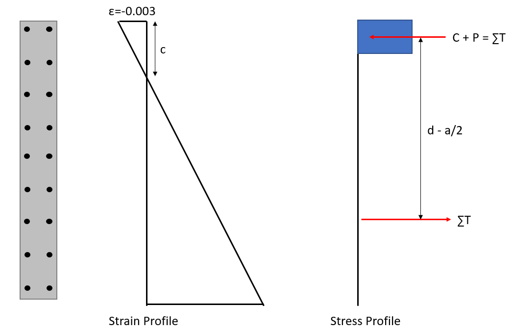
In the case of a uniformly reinforced shear wall, we can make an educated guess as to what the internal lever arm \(d-\frac{a}{2}\) might be. Assuming a very very small depth of neutral axis, the maximum possible lever arm possible is half the wall length:

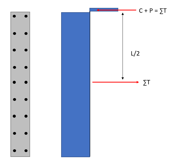
The actual internal lever arm is a certain fraction “j” of this maximum lever arm. We can make j a function of neutral axis depth (c).

The above equation for “j” makes sense.

• If c = L, at full compression capacity, then j = 0 and jd = 0 and M = 0
• If c near 0, we have the maximum lever arm, j = 0.5L

Combining everything above, we have this equation:

Derivation Part 2: Neutral Axis Depth

Next we need a way to predict depth of neutral axis. We can use the following equation:

We need to somehow modify the \(\sum T\) term because we cannot assume all reinforcing steel have yielded. A good modifier is shown below.

• if c = L, (1-2c/L)=-1, section is in full compression, steel is actually under compression => \(-f_yA_s\)
• if c = 0, (1-2c/L)=1, section is in full tension, => \(f_yA_s\)
• if c = 0.5, (1-2c/L)=0, section is half in tension, half in compression => no net force from reinforcing steel.

Isolate and solve for “c”:

Derivation Part 3: Adding Boundary Elements

Shear walls usually have concentrated reinforcement at the ends known as boundary elements. These areas of concentrated steel can be treated separately as a concentrated couple.

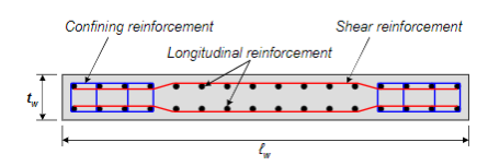
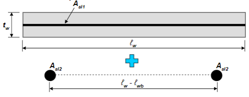
Therefore, the moment contribution from the two lumped steel area is:

Putting It All Together

Step 1: determine area of steel in web region of wall and in boundary elements, and other general wall information

• \(A_g\) = gross wall area
• \(A_{be}\) = steel area in one of the boundary element
• \(A_{web}\) = steel area in wall web region
• \(t\) = wall thickness
• \(L\) = wall total length
• \(L_{web}\) = wall length of web region
• \(L_{be}\) = length of boundary element
• \(\beta\) = rectangular stress block parameter per ACI 318
• \(P_u\) = Axial Load Demand

Step 2: adjust steel area because boundary steel and equivalent steel plate overlap. Increase web steel to extend into boundary region, and subtract this amount from the boundary steel.

Step 3: approximate depth of neutral axis. let

Step 4: determine moment capacity contribution from boundary element steel

Step 5: Determine moment capacity contribution from the equivalent steel plate

Step 6: Moment capacity at axial demand \(P_u\)

And voila, an approximate flexure+axial interaction equation that can be calculated by hand fairly quickly. Here is an implementation of it in python.

Please note that the approximation is limited to symmetrical planar walls without any irregularities.

def approx_PM(Pu,fy,lw,tw,fpc,lwb,lww,Ag,Aweb,Abe):   
    """
    parameter:
        Pu = axial demand
        fy = steel yield strength
        lw = length of wall
        tw = thickness of wall
        fpc = concrete compressive strength
        lwb = length of boundary element
        lww = length of wall web
        Ag = gross area of wall
        Aweb = area of web steel
        Abe = area of one boundary element steel
    return:
        Pn = axial capacity
        Mn = moment capacity
        c = depth of neutral axis

    Notation:
        Mn1 = moment contribution from BE
        Mn2 = moment contribution from web
        Fy = yield strength of rebar
        Pu = axial demand
        Aslb = area of steel in boundary element
        Aslw = area of steel in web
        Asl1 = area of equivalent steel plate
        Asl2 = area of boundary steel adjusted
        lw = length of wall
        lwb = length of BE
        lww = length of wall web
        tw = thickness of wall
        c = depth of neutral axis
        w = reinforcement ratio
        alpha = axial load ratio
        beta = stress block parameter
    """

    # step 2
    Asl1 = Aweb * Lw/Lww
    Asl2 = Abe - A_web * Lwb/Lww

    # step 3
    alpha = Pu/(fpc*Ag)
    
    if fpc < 4:
        beta = 0.85
    elif fpc > 8:
        beta = 0.65
    else:
        beta = 0.85 - 0.05*(fpc*1000-4000)/1000
        
    w = Asl1*fy/lw/tw/fpc
    
    c = (w + alpha) / (2*w+0.85*beta)*lw
    
    # step 4
    Mn2 = Asl2*fy*(lw-lwb)
    
    # step 5
    Mn1 = 0.5*Asl1*fy*lw*(1+Pu/Asl1/fy)*(1-c/lw)
    
    # step 6
    Mn = (Mn1 + Mn2)/12
    Pn = Pu
    
    return Pn, Mn, c

How well does it work?

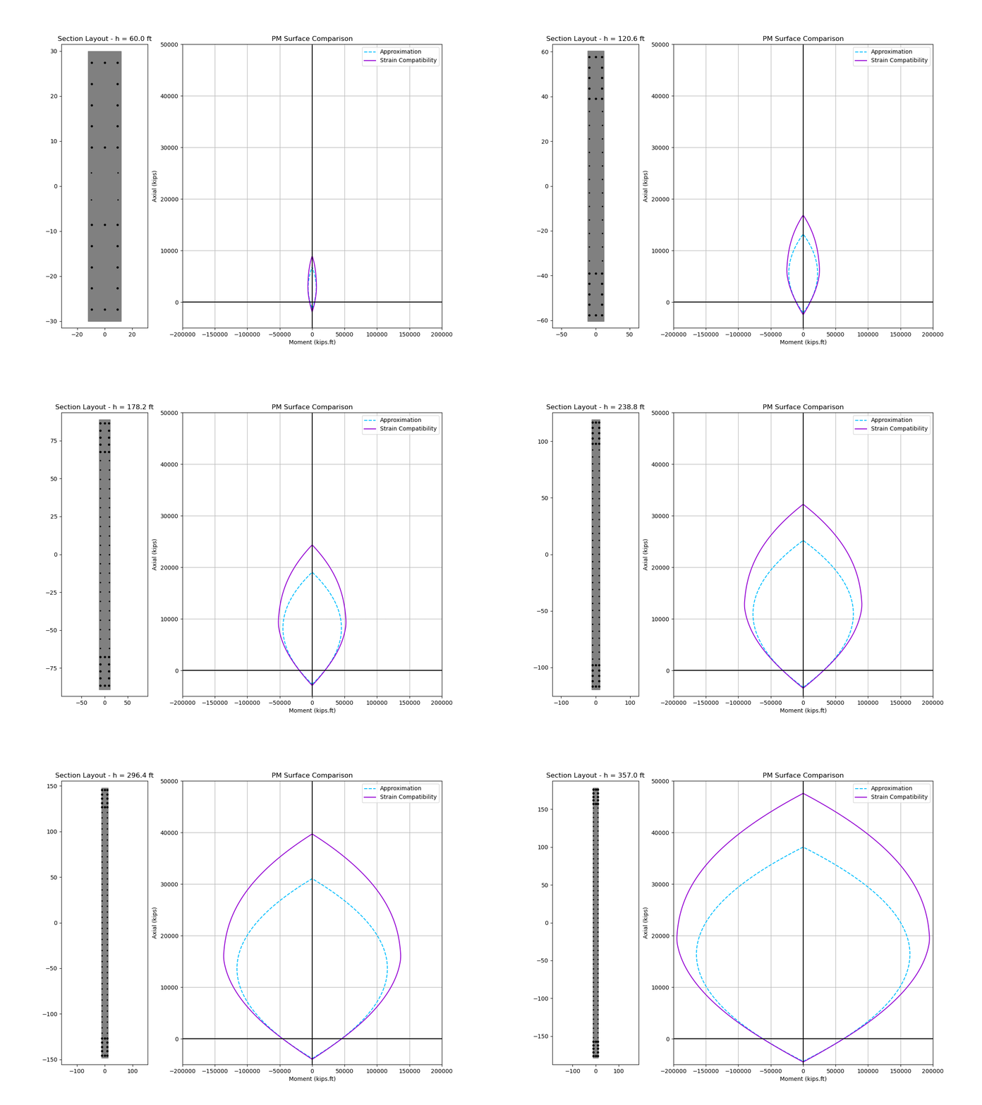
Here is an animated comparison of nominal interaction curve and depth of neutral axis between the approximate solution vs. strain compatibility analysis. The wall under consideration has typical design parameters:

• wall length ranges from 60 inch to 360 inch
• 6 ksi concrete and 60 ksi reinforcement
• 24 inch thick wall, 2 inch clear cover to reinforcement
• #6 @ 6” each way each face in web region
• 24 inch boundary element with (12) #10

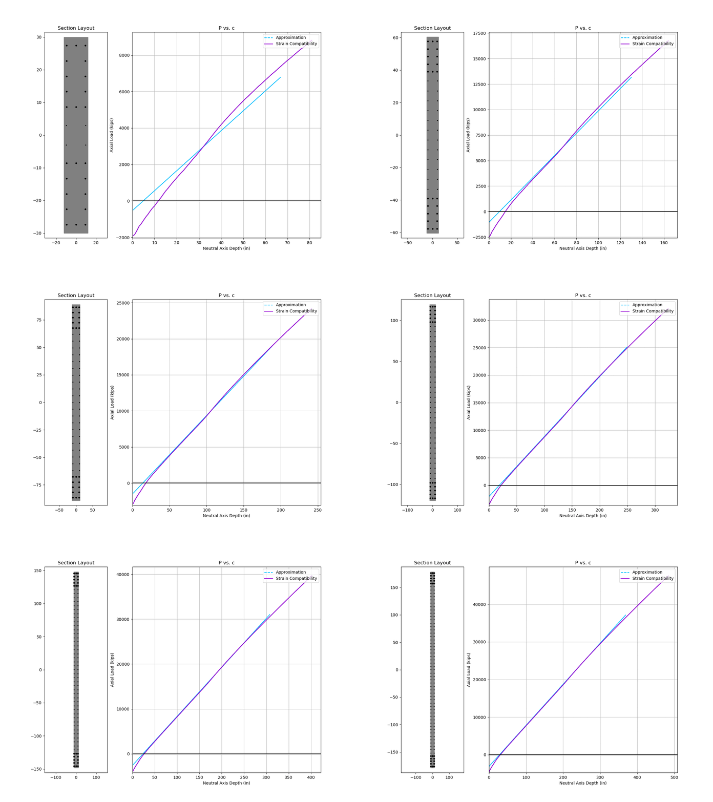Two things to note:

• The approximate solution is stupidly accurate for neutral axis depth (c)
• The approximate interaction curve is also surprisingly accurate except for high compressive strain near the top of the curve

The inaccuracy at high compression demand is reasonable given our assumption of yielded steel. To obtain a better fit near the top of the interaction curve, we may add in an adjustment factor \(\zeta\) to our equation in step 5.

Here is a typical shear wall with \(\zeta\) factor set to 0.83. Look how accurate you can get

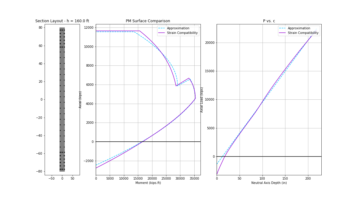
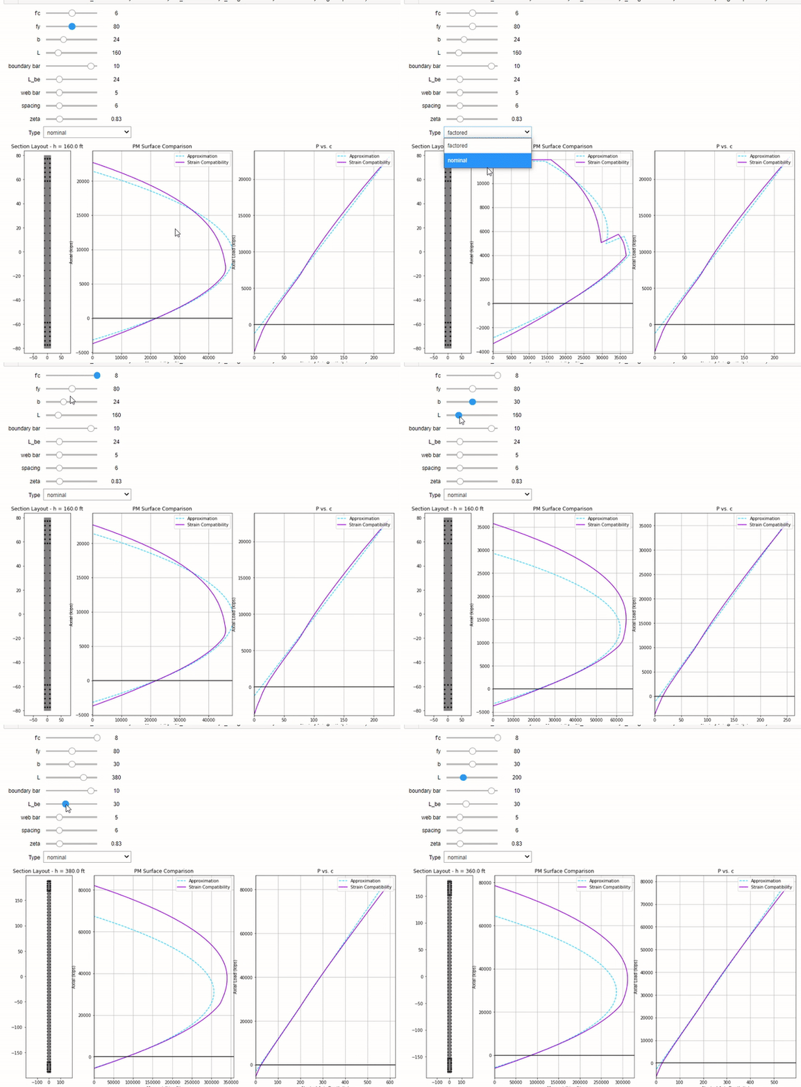
Admittedly this adjustment isn’t required as the solution is accurate enough and conservative. You can adjust \(\zeta\) to your liking, but I find values between 0.8 to 0.9 to work well for 6 ksi concrete and 60 ksi steel. Please note that \(f'_c\) and \(f_y\) seems to dramatically affect how well the fit is. Try for yourself. Perhaps it would be better to leave it at 1.0.

I made an interactive Jupyter notebook where you can use sliders to vary different design parameters. Take a look!

Download Notebook Here