Local and Global Axes

How Are Local Axes Defined in FEA Softwares?

Let global axis direction vectors be denoted by X,Y,Z, and let local axis direction vectors be denoted x,y,z. The algorithm for determining local axis of an element is as follows:

Given two nodes (starting node i, and end node j):

+x local axis:

+z local axis:

We are effectively enforcing the +y axis to always point skyward (up).

+y local axis:

The elements of the lambda vectors are direction cosines of your local axis (\(\alpha, \beta, \gamma\)). The 3x3 transformation matrix is defined as:

Rotate web-direction vector (+y) by angle beta:

Matrix multiply the above gamma matrices:

Finally, our element transformation matrix T can be defined as a 12x12 matrix with gamma on the diagonal. Let

Note that all direction vectors must be normalized to be unit vectors. Here is an example implementation that I wrote while developing MSApy.

def compute_T(end_nodes,beta):
    """
    parameter:
        end_nodes=[[xi,yi,zi],[xi,yi,zi]]
        beta = rotation of web-direction vector in degrees
    return:
        transformation matrix T
    """
    # Direction cosine in x-direction
    i_coord = np.array(end_nodes[0])
    j_coord = np.array(end_nodes[1])
    L = np.linalg.norm(j_coord - i_coord)
    position_vector = j_coord - i_coord
    cosinex = position_vector/L


    # Direction cosine in z
    if np.all(cosinex == [0,1,0]):
        cosinez = np.array([0,0,1])
    elif np.all(cosinex == [0,-1,0]):
        cosinez = np.array([0,0,-1])
    else:
        cosinez = np.cross(cosinex,np.array([0,1,0]))
        cosinez = cosinez/np.linalg.norm(cosinez)


    # Direction cosine in y (web-direction)
    cosiney = np.cross(cosinez,cosinex)
    cosiney = cosiney/np.linalg.norm(cosiney)


    # Beta angle rotation
    beta_rad = beta*math.pi/180
    gamma_b = np.array([
        [1,0,0],
        [0, math.cos(beta_rad), math.sin(beta_rad)],
        [0, -math.sin(beta_rad), math.cos(beta_rad)]])


    # Assemble gamma matrix
    gamma_p = np.zeros([3,3])
    gamma_p[0,:] = cosinex
    gamma_p[1,:] = cosiney
    gamma_p[2,:] = cosinez
    gamma = gamma_b@gamma_p


    # Assemble transformation matrix
    zero = np.zeros([3,3])
    T = np.block([
        [gamma,zero,zero,zero],
        [zero,gamma,zero,zero],
        [zero,zero,gamma,zero],
        [zero,zero,zero,gamma]])
    return T, gamma,L,cosinex,cosiney,cosinez

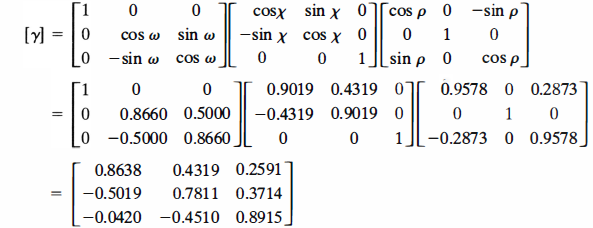
To verify, let do an example from the MASTAN textbook. Example 5.5. Using the code above, we get the same answer! Figure 6: Verification Problem

Note that the solution presented in the textbook is an alternative approach that uses the Euler angles to apply 3 sets of rotational transformation one after each other about the y, z’, and x’ axis (like a gimbal). Nevertheless the same answer is obtained.

Why Is it Good To Follow Conventions?

In FEM modeling, you may have been told to follow certain conventions when drawing elements (e.g. draw nodes counter clockwise, left to right, bottom to top, and etc.). There are good reasons for this, one of them is directly relevant to our discussion of local-axes.

First of all, not following convention won’t invalidate the analysis necessarily. Element nodal forces and displacements should still be correct because stiffnesses at each degree of freedom are mapped correctly regardless of member orientation.

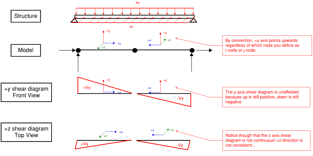
However, problems arise when you use any force plotting features such as for moment diagram, Von Mises stress, and etc. To illustrate, let’s say we have the following structure with directly opposing local axes.

Figure 7: Why Follow Conventions When FEM Modeling

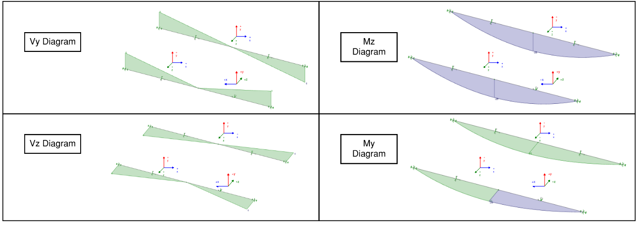
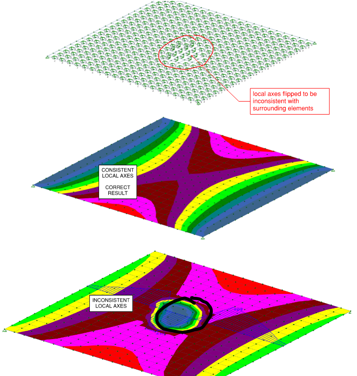
The fact that we enforce upward-facing web direction vector (+y) create situations where +z local axes are flipped and discontinuous if conventions are not followed. Let’s see this in action. Modeling the structure above in RISA-3D:

Figure 8: Line Element With Inconsistent Local Axes

Figure 9: Shell Element with Inconsistent Local Axes