Personal Python Handbook
In this notebook, I’ve gathered a whole bunch of code snippets that helps me along in my side projects.
- 1.0 Getting Started
- 2.0 Basic Syntax
- 3.0 Containers
- 4.0 File IO
- 5.0 Object-Oriented Programming
- 6.0 Numpy and Scipy
- 7.0 Sympy
- 8.0 Matplotlib
- 9.0 Pandas
- 10.0 Plotly
- 11.0 Images - Graphics - Animation
- APPENDIX A - Conceptual Stuff
- APPENDIX B - Styling Recommendation
- RANDOM NOTES
1.0 Getting Started
Programming Tips
- The most important skill in programming is breaking down (decompose) a large problem into smaller pieces. One common approach is to tackle the problem “top-down”. Outline the solution in abstract form and divide tasks into functions. You can call the function that you are going to write thus putting structure to your thought process
def main():
    a=task1()
    b=task2()
    task3()
- Always put concise comment. You will likely spend more time reading code than writing them
Installing Python
To get started, we need to install python. There are different ways of doing this but by far the most expedient way to install python along with hundreds of its useful packages is to install Anaconda. Think of it as a “battery-included” version of python with most of the popular packages.
For more advanced users, you can install python by itself here: python installation. Python comes with a set of standard packages which include useful things like math, json, subprocess, os, time, tkinter, etc. Refer to appendix A for more information on managing packages yourself and creating virtual environments.
Working with Python
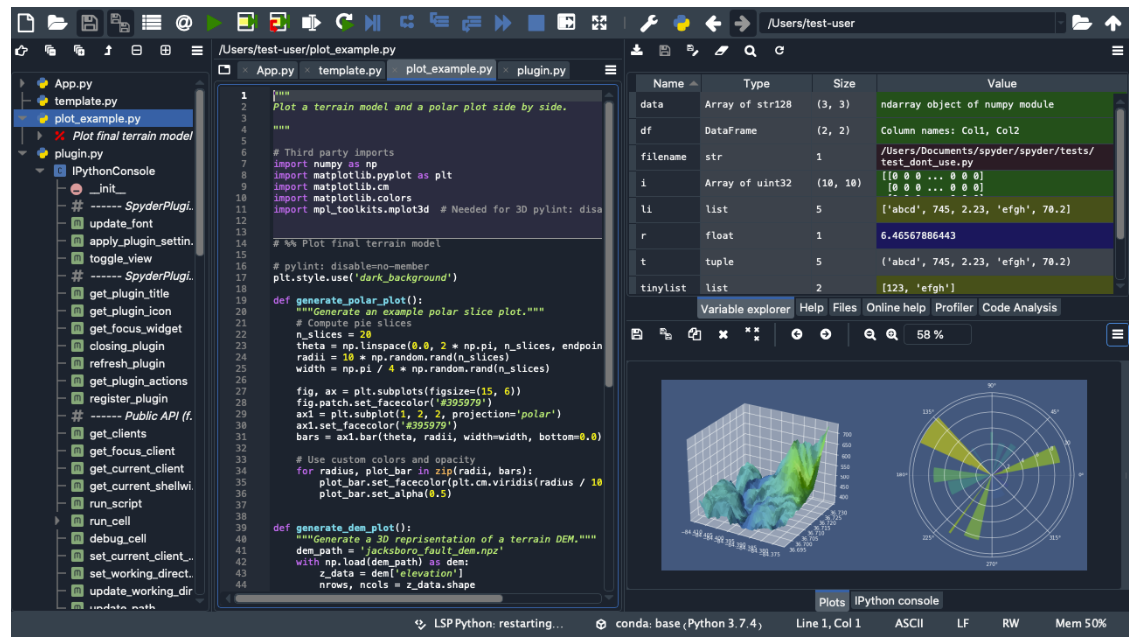
- Option 1: Write, debug, and run code from a Integrated Developer Environment (IDE). (Pycharm, Spyder, VSCode, etc)
- Spyder along with its Ipython console is most similar to Matlab’s REPL Interface (Read, Evaluate, Print, Loop), as well as a variable window to see all the variables you’ve defined in the namespace
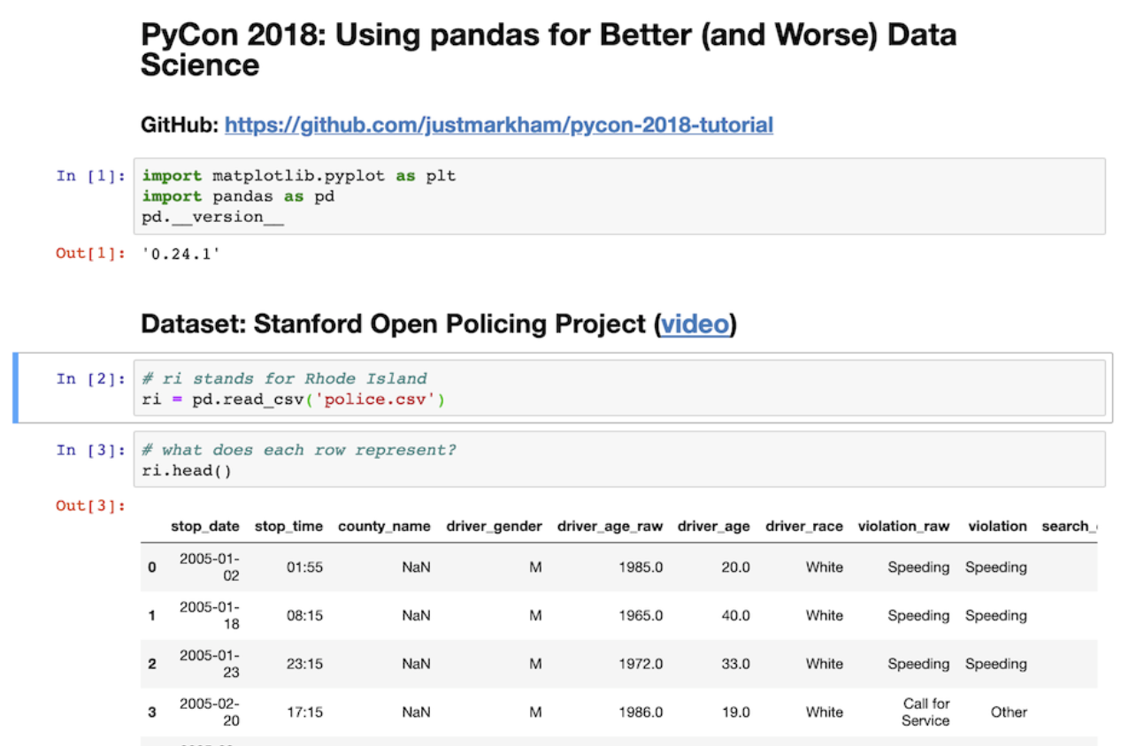
- Option 2: Work in notebooks like Jupyter Notebook, or Google Colab. This is most popular with Data Scientist because you can annotate and provide visualizations as you code (as if you are writing in a notebook)
- Option 3: Write code in a text editor like Sublime Text, then run script from Terminal (cmd, PowerShell, Bash, etc) as shown in the code snippet below
# FROM THE TERMINAL -------
python myscript.py arg1 arg2
# The above only works because "python" is added to PATH. Otherwise you need to write the full path:
"C:\Users\wcfro\AppData\Local\Programs\Python\Python311\python" arg1 arg2

# On windows, there is a dedicated python launcher called "py" which is preferred.
py myscript.py
# you can specify which version of python to use with py launcher
py -3.11 myscript.py
# if you run py within a virtual environment, it will run that version of python by default
# Here are some useful commands with py launcher
py -0p  # see all python installations on your machine and their path
py -0   # see all python installations and which one is default
# To change the default version of python used. Go to environment variable setting and change/add (PY_PYTHON=3.xx)

# WITHIN script.py ----------
# To receive arguments from the terminal, within python:
import sys

# Note that all inputs are strings initially! sys.argv[0] is myscript.py
user_input1 = int(sys.argv[1])
user_input2 = int(sys.argv[2])

# Handling exception where there is not enough input argument
if len(sys.argv) < 3:
    print("Not enough arguments")
    print("    $ python3 generatedata.py ref_file reads_file align_file")
    print("Example:")
    print('    $ python3 generatedata.py \"reffile.txt\" \"readsfile.txt\" \"alignfile.txt\"')
    sys.exit()
Note the difference between terminal and python console!
- Terminal - command line interface to interact with your computer
- Python console - what you get when you run python.exe
Installing Open-Source Packages
Here are the steps to go from an empty folder to a fully set-up python project environment
# 1.) Download the package you're interested in on github
git clone https://github.com/wcfrobert/SOMEPACKAGE.git

# 2.) navigate to that folder
cd SOMEPACKAGE

# 3.) Create a virtual environment stored in folder called "venv". This will contain python.exe as well as packages
py -m venv venv

# 4.) Activate environment:
venv/Scripts/activate

# 5.) Optional but you may want to upgrade pip
pip install --upgrade pip

# 6.) install from requirements.txt that most open-source developers will include
pip install -r requirements.txt

# 7.) if you want to install specific packages
pip install numpy

# 8.) list out all the packages. See if you are missing something
pip list

# 8.) Once you have everything. Test run some scripts
py main.py

# If you are using pycharm, go to the "Tools" drop down menu, click on "sync python requirements" to generate requirements.txt
# When you open a new project with pycharm, a tooltip should automatically pop up telling you to install stuff from requirements.txt


# Here are some other special commands
# If you need to exit the venv
deactivate

# Generate a requirements.txt for sharing with other people
pip freeze > requirements.txt

# check python or pip version
py --version
pip --version
The process is extremely similar if you are using Anaconda.
git clone https://github.com/wcfrobert/SOMEPACKAGE.git
cd SOMEPACKAGE
conda create --name my_env
conda activate my_env
conda list
# try to install everything you can with conda before using pip
conda install numpy
pip install -r requirements.txt
conda deactivate
Creating a New GitHub Repo
# 1.) Create project locally and enable git
    git init
    git add .
    git commit -m "first commit"

# 2.) Create empty repo on github ideally with the same name. Copy the .git link that's generated
    https://github.com/wcfrobert/YOURPACKAGE.git

# 3.) In your terminal, connect to remote repo
    git remote add origin https://github.com/wcfrobert/YOURPACKAGE.git

# 4.) Then push to Github
    git push -u origin master

# subsequent updates
git add .
git commit -m "a message"
git push origin master
Packaging a Project and Uploading to PyPi
# create a pyproject.toml and enter your project information inside the file

[build-system]
requires = ["hatchling"]
build-backend = "hatchling.build"


[project]
name = "package name"
version = "1.0.0"
authors = [
  { name="yourname", email="youremail" },
]
description = "short description"
readme = "README.md"
requires-python = ">=3.7"
classifiers = [
    "Programming Language :: Python :: 3",
    "License :: OSI Approved :: MIT License",
    "Operating System :: OS Independent",
]

[project.urls]
"Homepage" = "https://github.com/yourname/yourpackage"
"Bug Tracker" = "https://github.com/yourname/yourpackage/issues"


# package up files with build. Will create a folder called dist/
    pip install --upgrade build
    py -m build

# install twine which is an upload tool to upload to PyPi. Make sure you have an account
    pip install --upgrade twine
    twine upload dist/*
2.0 Basic Syntax
Code Structure
The basic code structure follows something like shown. Since any python code can be imported directly like modules, we use the structure below to prevent our code from running if imported.
For instance, say our script is called myscript.py. If we run it in the terminal, its “__name__” is “__main__” . If the script is imported, then the “__name__” is “myscript”.
# Have imports in alphabetical order if there are a lot
import numpy as np
import time

def main():
    print("your code in here")

def my_helper_function():
    print("functions can be anywhere. No need to define at top")


# Boiler plate. No need to modify
if __name__ == "__main__":
    time_start = time.time()
    main()
    time_end = time.time()
    print("Script completed. Total elapsed time: {:.2f} seconds".format(time_end - time_start))
else:
    print("{} Package imported!".format(__name__))
Basics
# Comment with # or triple quote """
# End lines that are too long with back slash \
if 1900 < year < 2100 and 1 <= month <= 12 \
   and 1 <= day <= 31 and 0 <= hour < 24 \
   and 0 <= minute < 60 and 0 <= second < 60:
        return 1


# Multiple variables can be assigned in one line via tuple unpacking
varA,VarB,VarC = 1,2,3
user_input = input("User can enter a value. Returned as string type")


# Printing (:.2f signals two decimal place float)
# Other types {:.2e} two decimal engineering
print('this is {:.2f} called {} string formatting'.format(varA,varB))
print("can assign names like this {name2}, {name1}".format(name1 = varA, name2 = varB))
print("or number them differently {1}, {0}".format(varA,varB))
print(f"the newest and preferred method in python is to use fstring : {var1}, {var2:.2f}")
# (:.1f) = two decimal place float (3.1)
# (:.2e) = two decimal engineering (3.14e+0)

print("print without moving to next line",end="")
print("print empty lines or tabs \n \t")

# Math operations. Integer automatically converted to float if there is another float
a+b, a-b, a*b, a/b
a**2		# exponent is NOT done using ^ but **
a//b		# floor division 5//2=2
a%b	        # modulo (remainder) 5%2=1
abs(a)		# absolute value


# Other math operation located in math module. For example:
import math
math.sin(x)
math.sqrt(x)		# or just use x**(1/2)
math.isclose(a,b)	# never compare two floats using ==. Use this instead
Functions
# Defining functions
def someFunction(arg1,arg2,arg3=defaultval,*kwargs):
	if condition:
    	return x,y,z
    else:
        return a,b,c
# Notice in the above function:
# - we can set default values
# - we can play around with return statement within ifs
# - we can return multiple values using tuple unpacking


# Sometimes we don't know how many arguments will be passed. We can define
# a function that accepts a variable number of arguments
my_sum(1,2,3,4,5,6,7,8,9,0,11,22,33,44)
def my_sum(*args):
    # *args can be many arguments. We might not known how many beforehand
    result = 0
    for x in args:
        result += x
    return result


# Sometimes a function might have a lot of arguments but we only care about a few.
# In these cases we can pass in keyword (named) arguments
concatenate(abc="Test", keyarg="Argument", somevar="Keyword", defw="Mapped")
def concatenate(**kwargs):
    print(kwargs["abc"])
    print(kwargs["keyarg"])


# Note that ordering matters. Need to specify unnamed args, *args, then **kwargs
def my_function(a, b, *args, **kwargs):
    pass
Flow Control
# If statements. The "pass" syntax is just a blank filler statement
if condition:
    pass
elif:
    pass
else:
    pass

# While loops
while condition:
    pass


# if n = 10, range(1) will run 10 loops from 0 to 9 by design
for i in range(10): #Loops from 0,1,2,...,9
    pass

for i in range(4,10): # Loops from 4,5,6,7,8,9
    pass # 10-4 = 6 loops

for i in reversed(range(3)): # Loop from 2,1,0
Raising Exceptions
# Raising Exceptions and Errors
if somecondition:
    raise RuntimeError('Mismatch dimension for pressure coefficient')

# try-exception flow control. Code within "try" will always run
try:
    step3=float(step2)
except ValueError:
    raise RuntimeError('wrong data type')
Importing Modules
# python code can be considered a module. When you import a module
# you are allowed to use all its defined functions

# Generic import (need to always use prefix). Only imports functions from module
import numpy as np
np.array(mylist)

# Function import - import only the function you need. Don't need prefix
from math import sqrt # OK BUT NOT RECOMMENED
sqrt(25)

# Universal import - Akin to a giant copy-paste running the code in module on line 1.
# All variables in mymodule namespace gets copied over. Say the module you are
# importing also imports moduleX. You will now have access to moduleX as well
from mymodule import * # NOT RECOMMENDED
3.0 Containers
Working with containers is probably the most important skill to have. There are four main types of containers:
- List [] - Ordered and mutable (can be modified). Lists are used when you want to easily append or index
- Tuples () - Ordered list can is immutable (cannot be modified). Cannot assign any value to a tuple index
- Sets {} - Lists with only unique elements. Use when we care about existence but not duplicity. It is also useful for finding intersection/union of two sets
- Dictionaries {} - Conventionally referred to as a map. It is a key-value pair. Order is not guaranteed and you should NEVER try to sort or index a dictionary. If you are, there is probably a better way to approach the problem.
- Strings “” can also be thought of as a container of characters. Indeed, indexing a string is exactly the same as indexing a list.
Lists
# Fundamentals
myList = []
mylist.append('new item')
mylist[index]='index with square bracket'

# Unique python behavior. Assigns list by reference
a = [1,2,3]
b = a
b[0] = 99
# In the code above, Both a and b points to the same list in memory.
# changing b also changes a. To avoid this
b = a.copy() # Copy a separate instance


# Finding things in list (first occurence)
index = mylist.index(elementimlookingfor)

# Checking existence of something in a list
if element in list: 	#check existence with python "in"

# Adding and removing elements from list
a = mylist.pop() 	# return last element and returns it (also modifies the list)
a = mylist.pop(3) 	# pop element in index 3
mylist.remove(element) 	# remove first occurence
del mylist[0:4] 	# use to remove a slice of list
list1.extend(list2) 	# append list2 to list1
list3 = list1 + list2 	# this is the simpler way to accomplish the same thing
list1.insert(index,val) #val becomes element at index. Everything else pushed back

# Other useful operations
mylist.sort() 		# sort in increasing order
random.choice(list) 	# returns a random item from list
mylist.reverse() 	# reverse a list. First item becomes last
max(list), min(list), sum(list)


# List Comprehension is very useful when you want to perform operations on all
# element of a list in a very compact manner
squaredlist = [x*x for x in mylist]
filteredlist = [x for x in mylist if x>2==1]

# subtract every item in the list by Y
[x - Y for x in ListA]

# Given two list, multiply elementwise
[a*b for a,b in zip(ListA,ListB)]

# Extract only the unique items from a list
list(set(originallist))

# Checking if list is empty
if len(list):
    pass

# Sets, strings, dictionaries, tuples can all be converted to list
list(myset), list(string), list(tuples), list(mydict.values())
Strings
String operations are sometimes called “parsing” strings. It is one of the most common tasks in programming. Mastering string parsing will also translate to a mastery of operating with lists.
# String Slicing
mystr='abcdefghijklmn'
mystr[1] 		# returns b
mystr[4:8] 		# returns efgh
mystr[:4] 		# returns abcd (first 4 letters)
mystr[4:] 		# returns efghijklmn (everything after first 4 letters)
mystr[-4:] 		# returns klmn (last 4 letters)
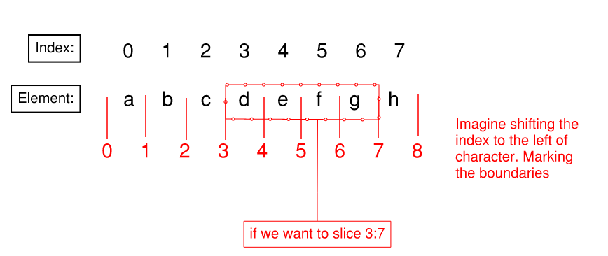
"""
The trick is to picture index on the left of char. Imagine boundary line on left
 a b c d e f g h
0 1 2 3 4 5 6 7 8
We want to make cut at 4 and 8. Leaving us efgh

Since string is just a list of characters. The above operation also works on lists
"""

# Note that strings are immutable and when you use a string method, you must
# assign it to another variable. The original string is not affected.
newstring = mystring.split()	# does not affect mystring
mystring[3] = "a"				# THIS IS NOT ALLOWED


# Other useful string operations for parsing
concat = str1 + str2		# concatenate strings
"word" in string		# checks if "word" is in the string. Returns boolean
string.find("word")		# find the index where "word" occurs. Returns -1 if failed
string.strip() 			# removes spaces and \n \t
string.strip(",.abc:;") 	# remove occurence of these characters
string.split(" ") 		# Split into list of strings at white space
string.split(",") 		# Split into list of strings at comma or any other character
string.count("word")		# count how many times substring "word" occured
string.uppercase()		# convert all to uppercase
string.lowercase()		# convert all to lowercase
string.swapcase()		# swap lower and upper case. Vice versa
string.startwith("2020")	# see if string starts with prefix "2020"
string.endswith(".jpeg")	# see if string ends in suffix ".jpeg"
The figure below illustrates a good way of thinking about list/spring slicing in Python:
Dictionaries
# Dictionaries are key-value Pairs. Key must be unique, value doesn't have to be
# Basics
myDict = {}
myDict['key1']=123123
myDict = {
    'key1':123
    'key2':223}
myval = myDict['key1']

# To look through dictionaries. ORDER NOT GUARANTEED!!!!! Things might shuffle around
for key in myDict.keys():
    pass
for value in myDict.Values():
    pass
for k,v in mydict.items():
    pass

# Other useful methods
mydict.items()				# return tuples of key-value pair
mydict.values()				# return values
mydict.keys()				# return keys
list(mydict.values) 		    # create a list of keys or values
'key' in dict 				# returns boolean indicating presence of key in dict
mydict[key1]=None 			# if you want to disassociate a value to key
mydict.pop(key) 			# remove entire key-value pair
del mydict[key]				# remove entire key-value pair
Tuples
# Tuple are just lists that cannot be modified nor appended
myTuple = (1,2,3)

# Tuple unpacking - assigns two variables at once. This is useful when
# a function returns multiple variables
mytuple = 4,5
var1,var2 = mytuple

def func():
    return a,b
var1,var2 = func()
Sets
# Sets are kind of like list, but they only contain unique entries
myset = set(myList)
myset ={1,2,3}

# Can use intersection of sets or union of sets
iteminboth = set(setA & setB) 		# Intersection
itemineither = set(setA | setB) 	# Union

# Other methods
myset.add()			# appending value to set
difference(set1,set2) 		# returns value that only occur in set1 but not set2
issubset(set1,set2)		# Check if set1 is subset of set2
issuperset(set1,set2)		# Check if set1 is superset of set2
discard(set1,set2) 		# Discard element from set1 if it exists in set 2
4.0 File IO
Reading and Writing
One thing to always remember is that all data read will be in string format.
# Reading data in columns from File
with open('file.txt', 'r') as f1:
    firstline = next(f) # skip first line
    secondline = next(f) # skip to second line
    Col1=[]
    Col2=[]
    Col3=[]
    for lines in f1: # Loop through each line
        split_data = lines.split() #split line
        Col1.append(float(split_data[0])) #extract column 1 data
        Col2.append(float(split_data[1])) #extract column 2 data
        Col3.append(float(split_data[2])) #extract column 3 data

# Read entire file in one go. Get a list of all lines
linesdata=f1.readlines()

# Writing to File
with open(outputfilename,'w') as f2:
    for items in mylist:
        f2.write('{},{},{}\n'.format(items[0],items[1],items[3]))
Managing Working Directories
import os

# get current working directory
os.getcwd()

# get path where the *.py file is stored
home_dir = os.path.dirname(__file__)

# list out all files
file_list = os.listdir(path)

# get all files of a specific format
png_list=[]
for f in file_list:
    if f.endswith(".png"):
        png_list.append(f)

# change directory
os.chdir("/scripts")

# make a new directory
os.mkdir("new_folder")

# check if directory exists
os.isdir()

# joining path
file_path = os.path.join(os.getcwd, "scripts", "file.csv")
Paths
Windows based operating system uses backslash () whereas unix based system use forward slash (/).
# need to escape back slash in python. Can do it in two ways

# double backslash
path = "E:\\data\\telluride\\newdata.gdb\\slopes"

# raw string
path = r"E:\data\telluride\newdata.gdb\slopes"

# using os.path to handle anything path related
path = os.path.join(os.getcwd(), "anotherfolder")
You may specify relative or absolute file paths
# Absolute path
pd.read_csv(r"C:\Users\wcfro\data.csv")

# Relative path. Use os.path.join. Never write out path yourself
dirname = os.path.dirname(__file__)
os.path.join(dirname, "subfolder/files/something.png")

# go back one folder (can use repeatedly)
parent_dir = os.path.dirname(child_dir)

# Not specifying any path
pd.read_csv("data.csv") #assuming file is in current working directory
Running a python script with Excel VBA
Spreadsheet modifications can be performed with pandas, openpyxl, xlwing. These all come pre-installed with the Anaconda distribution. Currently, it seems like only xlwing has the ability to modify spreadsheets “in real time” when you have it open.
- excel VBA –> bat file –> python script
# create a .bat file with the following
call C:\Users\%USERNAME%\anaconda3\Scripts\activate
python "%~dp0\myscript.py"
cmd \k

# first line activates anaconda venv which allows us to use packages
# second line calls the python script "myscript.py" in the same directory as the bat file
# third line makes sure the command line remains open after running

# within excel, create a macro that opens the .bat file
Sub runPythonScript()
status = Shell(ActivateWorkbook.Path & "\myscript\myscript.bat", vbNormalFocus)
End Sub
5.0 Object-Oriented Programming
Up until now, all of our programs have been Procedural. The code runs from top to bottom and jumps into functions as needed. However, this style of coding is ill-suited for larger and more complex programs. It is not scalable. At some point, the program becomes too big to manage. Hence why we need Object-Oriented programming (OOP).
What is Object-Oriented Programming?
- Object-Oriented programming is just another way of organizing data and logic. We create objects that contains data and behavior, and the program is the interaction of these objects. Here are some key definitions:
- Class - Template or blueprint for an object (e.g. BeamElement)
- Object - Instance of a class. (e.g. beam42)
- Method - Functions related to an object (e.g. beam42.calculate_Mp())
- Attributes - Variables related to an object (e.g. beam42.length)
- Dot Notation - The way in which we interact with objects
Why OOP?
OOP paradigm allows for better organization of data and logic, and promotes thinking at a “higher level of abstraction”. To give a very simple example:
# rather than writing something like:
y[2] = y[2] + 0.03
x[2] = x[2] + 0.04
color[2] = "green"

# we can start using higher abstraction and logic (easier to read and interpret)
ball3.move(0.04,0.03)
ball3.set_color("green")
Of course you would still have to define the method: “move()” and “set_color()”, but one is much easier to understand. You can start thinking bigger and more abstractly: “move the ball 0.04 units right, 0.03 units up”, rather than worrying about indexing an array and modifying the element that stores x-coordinates, etc.
Abstraction is a process of hiding unnecessary complexity and implementing more and more complex logic on top.
- High Abstraction = less detail, more general
- Low Abstraction = more detail, the nitty gritty stuff
What are the pros and cons of OOP?
Advantages
- Abstraction - Allows one to think at a higher level and build increasingly sophisticated programs. Often more intuitive.
- Encapsulation - The internal complexity of a class is hidden away from the user (e.g. I can make coffee without knowing how a coffee machine works).
- Collaboration - It is much easier to partition work when collaborating with other programmers on a big project. Code is modularized.
Disavantages
- Initial learning curve
- More boiler plate code
- if not well-design, code is more obfuscated and difficult to understand
Example
When an object is instantiated, the commands within the constructor runs first.
# Typical class definition. Note places where "self" is required
class myclass:
    def __init__(self,arg1,arg2):
        self.property1=arg1
        self.property2=self.ComputeLength(arg2)
        # Private properties are defined with double underscore
        # This is just a trick through variable obfuscation. Everything is public in python
        self.__privateproperty = inputarg2

    def ComputeLength(self,arg2):
        return self.property1*arg2

# Create instance of class with:
myobject = myclass(arg1,arg2)
a.property1
a.ComputeLength

# inheritence
class class1(myclass):
    pass
6.0 Numpy and Scipy
If you are already familiar with Matlab. This quick start guide is all you need: https://numpy.org/doc/stable/user/numpy-for-matlab-users.html. If a command exists in Matlab, it will likely also exist in numpy; often with the same syntax. The tricky thing to get used to is 0-based indexing and slicing!
Importing
import numpy as np
import scipy as sp
import scipy.sparse
import scipy.sparse.linalg
Basic Commands
"""
All matrices and vectors are considered np.arrays.

If an array is one-dimensional. Numpy does not make a distinction between column or row vector
It's 1-D shape will be adjusted automatically to whatever is workable. Of course, you can force
an array to be column if needed by putting more square brackets.
"""

# Creating arrays
mylist = [1,2,3,4,5]
A = np.array(mylist)
M = np.array([
    [1,2,3],
    [4,5,6],
    [7,8,9]
])

# Create random arrays or matrices
np.random.rand(m,n)		# element number from 0 to 1 uniform dist
np.random.randn(m,n)	# element number from 0 to 1 normal dist
np.randint(a,b,(m,n))	# integer from a to b

# Uniformly spaced array. Used for plotting.
# Create an array from i to j in N steps
x = np.linspace(i,j,N)

# Elementwise operations
A + 3.1415		# adding a scalar
A + B			# elementwise addition
A - B			# elementwise subtraction
A * B			# elementwise multiplication
A / B			# elementwise division
np.sqrt(A)		# elementwise squareroot
A**2			# elementwise squared

# Matrix multiplication with @
A @ B

# Other useful operations:
A.sum()			# sum of all elements
A.shape()		# checking shape of array
A.T()			# transpose of the matrix
np.eye()		# identity matrix
np.one((m,n))		# matrix filled with 1
np.one((m,n))*N		# matrix filled with N
np.zero((m,n))		# matrix filled with 0
# https://numpy.org/doc/stable/user/numpy-for-matlab-users.html for more
Indexing and Slicing
Python uses 0-based indexing which may take some getting used to if you are proficient in Matlab already. In the case of indexing a single element, you just need to remember to subtract by one for each index.
# For single index. Just subtract by one. e.g. for the (2,3) element of A
A[1,2]

# For last element, use -1
A[-1]

# For an entire column or row
A[:,0]		# first column
A[3,:]		# fourth row
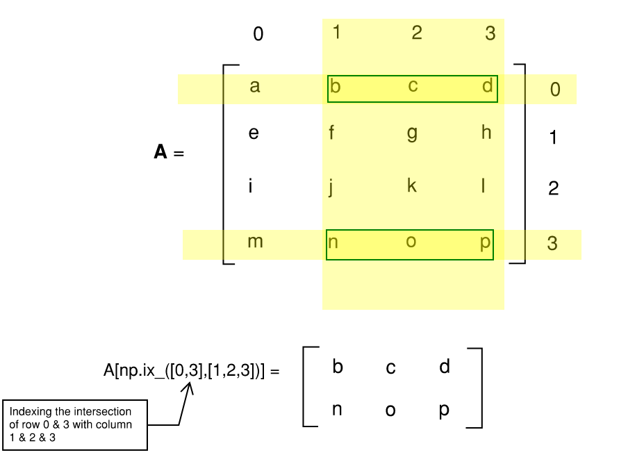
Slicing works differently. When slicing from A to B, A is inclusive whereas B is not! Let’s do an example:
\[A= \begin{bmatrix} a&b&c&d \\ e&f&g&h \\ i&j&k&l \\ m&n&o&p \\ \end{bmatrix}\]For instance, let’s say I want to extract the sub-matrix \(\begin{bmatrix}g&h\\k&l \end{bmatrix}\)
Meaning row 2->3 and column 3->4. In Matlab, it’s fairly intuitive A(2:3, 3:4). In python, we need to use A[1:3, 2:4]. Remember the end value of the range is not included in Python. Therefore; you are subtracting by 1 for the start value, but NOT subtracting for the end value. All of this is very confusing but gets better the more you work with arrays in Python. Here is an illustration that could potentially clear things up a little.
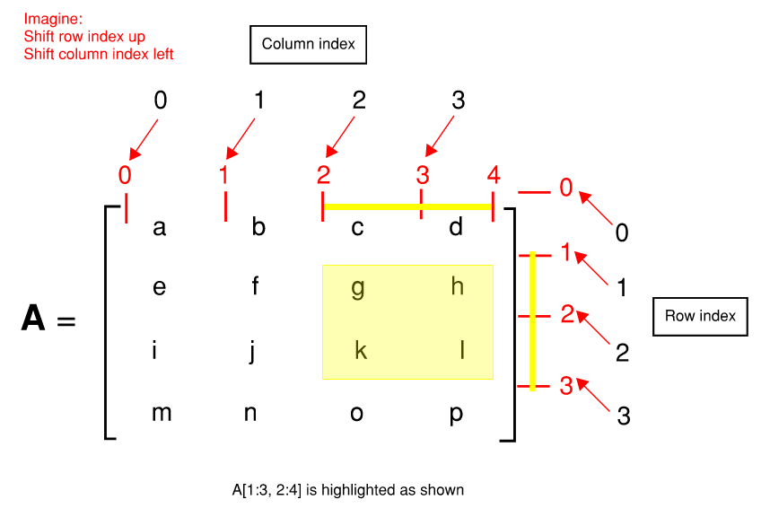 Figure: Illustration Showing Indexing of Matrices
# Notice we need to add .copy() to pass a copy rather than a reference
a = A[1:3,:].copy()		# second to third row
a = A[:,1:2].copy()		# is actually equivalent to A[:,1].
a = A[:,1].copy()		# however, this returns a flexible numpy array rather than a col vector

# Mesh indexing (e.g. in Matlab A([2,4,6],[1,3]))
A[np.ix_([1,3,5],[0,2])]
Additionally, we can create sub-matrices by passing to it list of index. This process is illustrated in the figure below:
Other Common Operations
# Finding max/min value within row or column
a.max()		        # returns scalar. Max in entire matrix
a.max(0)	        # returns vector. Max in each column
a.max(1)	        # returns vector. Max in each row
a.max(0)[2]	        # returns max in third column

# Returning index of value matching a certain condition
np.nonzero(a<3)		# returns i,j coord of element matching condition

# Appending to matrices in blocks
np.hstack((a,b))	# stack two column vector. b to the right of a
np.vstack((a,b))	# stack two row vector. b below a

# Say we want to stack four 2x2 matrices
np.block([
    [a,b],
    [c,d]
])
7.0 Sympy
All assignments are passed by value. In other words. A.changesomething() does not alter the memory location where A is stored. Instead, an entire copy is created that you assign to another variable.
Basics
# Initiating symbols
A,B,c,d,e = sy.symbols('A B c d e')

# At this point, all of the symbols can be used as variables
# If you are using say Jupyter Notebook. The output will render
# and show up nicely
A = B + C

# Integrating and differentiation
sy.integrate(f, (x,a,b))	# integrate f(x) from a to b
sy.diff(f,x)			# differentiate f(x) with respect to x

# symbolic matrix or vector
sy.Matrix([
    [a,b],
    [c,d]
])

# Solving. First rewrite expression with one side = 0
f = 2*x**2 + 3*x - 13
sy.solveset(f,x)
Substitution and Simplifying
# Simplifying
sy.simplify(f)

# Substitution
f2 = f.subs([(a,10),(b,22)])        # substitute a=10 and b=22
sy.N(f2)                            # convert symbol to float
f2.evalf()                          # another way of doing the same thing
Note that all variables stay a “symbol” even if you have already substituted everything. For instance, f = a + b. Both a and b are equal to 10. Then f = 20. At this moment the number 20 is actually still a symbol until you use sy.N() or .evalf().
Plotting
import sympy as sy
from sympy.plotting import plot3d
x, y = sy.symbols('x y')
plot3d(sy.cos(x*3)*sy.cos(y*5)-y, (x, -1, 1), (y, -1, 1))
8.0 Matplotlib
Matplotlib is an open-sourced python package used for creating plots. It was designed with Matlab users in mind to cater to a easy transition. See here for the official quickstart guide: https://matplotlib.org/stable/tutorials/introductory/pyplot.html
Most of plotting does not involve some tricky programming puzzle. It usually comes down to finding the correct syntax, the relevant parameters, the right examples; which usually means a lot of googling and reading through documentations.
Object-Oriented Approach vs. Pyplot Functional Interface
There are two methods of plotting with matplotlib:
- Object-oriented (preferred method)
- each plot is an object that can be accessed with standard dot notations
- objects can be viewed in variable explorer
- can easily manage multiple plots
- (e.g. axs.plot() where axs is our plot object)
- Pyplot functional interface (old method set up to imitate MATLAB)
- like a terminal where we input commands to change the current plot
- if you have multiple plots, need to switch back and forth
- (e.g. plt.plot() where plt is a command)
All contents hereafter will use the object-oriented approach.
Refer to this article for more information: https://matplotlib.org/matplotblog/posts/pyplot-vs-object-oriented-interface/.
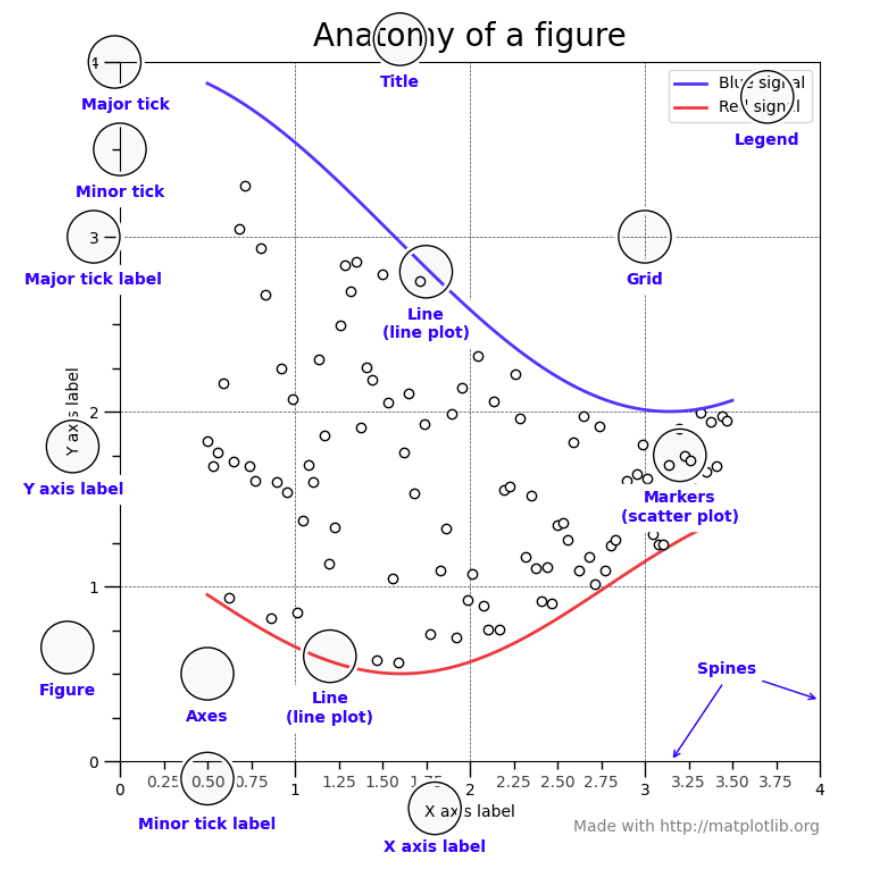
Initializing a Figure
import matplotlib.pyplot as plt
plt.ioff() #if you want to stop IDE from showing plot

# Basic single plot
fig, axs = plt.subplots() # figure can have multiple axes

# Multiple subplots - 3 vertically stacked
fig, axs = plt.subplots(3)

# Multiple subplots - 3 horizontally stacked with adjustable width
fig, axs = plt.subplots(1,3, gridspec_kw={"width_ratios":[2,2,3]})
# as of matplotlib 3.6+, width_ratios and height_ratios can be passed directly to subplots

# some useful arguments when initializing figure
fig, axs = plt.subplots(figsize=(11,8.5), dpi=100, ="white", edgecolor="white")


# Older method. More control with adding axes
fig = plt.figure()
fig.set_size_inches(9,6)
axs_1 = plt.axes([0.08,0.35,0.42,0.58]) #left-x, bottom-y, width, height
axs_2 = plt.axes([0.54,0.35,0.42,0.58])
axs_3 = plt.axes([0.08,0.1,0.88,0.2])
Plotting
# in the example above, axs is a tuple containing three axs objects. To plot in them:
axs[0].plot(x,y)
axs[1].plot(x,y)

# alternatively, you assign axes to individual variables
fig, (first_axs, another, axs3) = plt.subplots(3)
first_axs.plot(x,y)

# 2-D grid of subplots
fig,axs = plt.subplots(2,2) # index axs as you would with a 2D array


# plotting directly from pandas dataframe
axs.plot("HEADER1", "header2", data=my_df)

# basic plotting
axs.plot(x, y, label="label for legend",marker=".",c="forestgreen", markersize=9)
axs.plot(-x, -y, "-g", label="another line") # -g stands for green solid line
axs.plot([0],[0]) # even if you are plotting one point, needs to be a list


# some other useful arguments
axs.plot(x, y, label = "dataset1",
         color = "cornflowerblue",
         linestyle = "--",
         linewidth = 2,
         marker = "o",
         markeredgecolor = "black",
         markeredgewidth = 1,
         markerfacecolor = "red",
         markersize = 4,
         visible = True,
         zorder = 2)

"""
Common line styles:
    "." = point
    "o" = circle
    "v" = triangle
    "s" = square
    "*" = star
    "P" = plus
    "X" = cross

Common marker styles:
    "-" = solid
    "--" = dashed
    "-." = dashdot
    ":" = dotted
    "none" = don't draw lines
"""

# Named colors: https://matplotlib.org/stable/gallery/color/named_colors.html
# Other ways to specify color: https://matplotlib.org/stable/tutorials/colors/colors.html
# line styles: https://matplotlib.org/stable/api/_as_gen/matplotlib.lines.Line2D.html#matplotlib.lines.Line2D.set_linestyle
# marker styles: https://matplotlib.org/stable/api/markers_api.html#module-matplotlib.markers
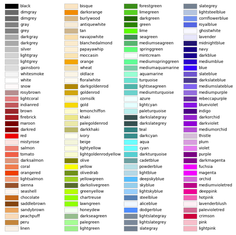
There are many other types of plots all covered here: https://matplotlib.org/stable/plot_types/index.html
Styling Basic
# show grid
axs.xaxis.grid(color="gray")
axs.yaxis.grid()

# add axis labels
axs.set_ylabel("time (s)", fontsize=14)
axs.set_xlabel("y value (km)", fontsize=14)

# add plot sub titles
fig.suptitle("Title. Can insert latex too: $\alpha_{a} > \frac{a}{b}$",fontweight="bold")

# Add legend
axs.legend(loc="upper left")
axs.legend(loc="best")

# set axis limit
axs.set_xlim([db_list[0],db_list[-1]])
axs.set_ylim(0,max(ld_4ksi)*1.1)

# make plot aspect ratio equal
axs.set_aspect('equal', 'box')

# put axis below any patches and data
axs.set_axisbelow(True)

# put a solid black line on x and y axis
axs_drift.axhline(y=0, color='black', linestyle='-', lw=0.8)
axs_drift.axvline(x=0, color='black', linestyle='-', lw=0.8)

# make x-tick label something else
value_list = [1,2,3,4,5,6,7,8,9]
label_list = ["#3","#4","#5","#6","#7","#8","#9","#10","#11"]
axs.set_xticks(value_list)
axs.set_xticklabels(label_list)

# saving figure
fig.savefig("my_plot.png") # can also save as pdf!

# showing figure
plt.close(figure2)
plt.show()
Annotation
# free form annotation anywhere on figure
axs.annotate("Disclaimer: this figure is cool", (600,380), xycoords='figure points', fontsize=14)

# annotate on data
axs.annotate("t = {:.1f} kips".format(t[i]), xy=(-xi[i], t[i]), xycoords='data', xytext=(10, 10), textcoords='offset points')
Producing Animation Frames
for i in range(len(N_frames)):
    # create figure
    fig, axs = plt.subplots()

    # save frames. Numbering is important for imagemagick
    fig.savefig("gif_folder\frame{:04d}.png".format(i))

    # then in command line with ImageMagick:
    # magick -delay 20 -loop 0 *.png mygif.gif
9.0 Pandas
Some Common Operations
# remove specific rows by index
df.drop([0,3,5,6,7])

# remove specific columns by index
df.drop(df.columns[[0,2,4]], axis = 1)

# remove specific columns by name
df.drop(columns=["header1","header2"])

# remove first row and convert it to the header
headers = df.iloc[0]
df = df[1:]
df.columns = headers

# Adding a new column to dataframe
df["new_column"] = 5 # you will get a column of all 5s

# read excel or csv without making first row into header
pd.read_csv(filepath, header=None)

# drop all nan values in dataframe
df.dropna()

# replace nan value with something else in the dataframe
df.fillna("new value")

# reset index after manipulating dataframe
df.reset_index()
Indexing Dataframes
# Label-based indexing with .loc
df.loc[4, "headerA"] #index 4, headerA. Note index don't have to be integers

# integer-based indexing with .iloc
df.iloc[2,4] #third row, fifth column

# Dataframes can be sliced like 2D arrays with .iloc
df.iloc[1:,2:8] #everything after first row, from column 2 to 7

# Slicing entire column
df.headerA
df["headerA"]
df.loc[:,"headerA"]
df.iloc[:,0]

# Slicing entire row
df.iloc[2,:]
df.loc["row1",:]

# mesh indexing
df.iloc[[0,2,4],1:3]
Querying Dataframes
# Method 1: boolean filter
df = df[df["headerA"]>2]
df = df[  (df.A=="normal")&(df.B=2)  ] # inner expression returns a long list of True/False

# Method 2: query function
df = df.query(f'headerA == "something" & headerB == "{varB}"')
10.0 Plotly
Introduction
Under the hood, all plotly figures are json files (dictionaries). You can actually convert them back and forth like so:
fig.to_json()
fig.to_dict()
If you peak under the hood:
Figure({
    'data': [{'hovertemplate': 'x=%{x}<br>y=%{y}<extra></extra>',
              'legendgroup': '',
              'line': {'color': '#636efa', 'dash': 'solid'},
              'marker': {'symbol': 'circle'},
              'mode': 'lines',
              'name': '',
              'orientation': 'v',
              'showlegend': False,
              'type': 'scatter',
              'x': array(['a', 'b', 'c'], dtype=object),
              'xaxis': 'x',
              'y': array([1, 3, 2]),
              'yaxis': 'y'}],
    'layout': {'legend': {'tracegroupgap': 0},
               'template': '...',
               'title': {'text': 'sample figure'},
               'xaxis': {'anchor': 'y', 'domain': [0.0, 1.0], 'title': {'text': 'x'}},
               'yaxis': {'anchor': 'x', 'domain': [0.0, 1.0], 'title': {'text': 'y'}}}
})

At the most basic level, a figure can be represented by the following hierarchy of attributes; each of which has their own sub attributes.
- Figure - a dictionary of three attributes:
- Data - raw data organized into a list of dictionaries. Each dictionary represents a subplot which is referred to as a trace. A trace can be one of more than 40 different plots (e.g. bar, scatter, scatter3d, pie, etc.)
- Layout - customize the look and feel of your figure. Organized as a dictionary containing various parameters you can tune. (e.g. title, legend, axis, fonts, hover, hover labels, annotations, etc.)
- Frames - used for animations. Organized as a list of dictionaries of data
As you can see, the data structure gets convoluted and you start having a dictionary of a dictionary of a list of dictionaries.
Rather than trying to index your way through a deeply-nested json, the recommended workflow is to create a graph object first, then using .add_trace() and .update_layout() to polish your figure step by step.
The plotly one-page reference https://plotly.com/python/reference/ is a must-have!
Styling with Magic Underscore
To change layouts, plotly has a nice feature known as “magic underscore”. In essence, the underscore automatically keys you in to the attribute you want. It is easier to explain through an example:
# Option 1: update layout with OOP dot notation
fig.layout.title.font.family = "Open Sans"

# Option 2: update layout with update method and magic underscore
fig.update_layout(title_font_family="Open Sans")
You can update many attributes at once, but the bracket matching can get confusing. More often than not, you are much better off tweaking one attribute at a time. For example:
# this:
fig.update_layout(title=dict(text="Base Reaction", x=0.5, font=dict(size=24)))

# is equivalent to this:
fig.update_layout(title="Base Reactions")
fig.update_layout(title_x=0.5)
fig.update_layout(title_font_size=24)
There are actually two ways to use Plotly:
- Quick and expedient way with plotly-express
- Object-oriented approach with graph-objects
My recommendation is to just start with graph-objects from the beginning.
Plotting Basics
# import
import plotly.graph_objects as go

# if you are having issue display plot in pycharm or spyder
import plotly.io as pio
pio.renderers.default = "browser"

# initialize figure
fig = go.Figure()

# add data
plot_data1 = go.Scatter(x=x, y=y, mode='markers', name="dataset1")
plot_data2 = go.Scatter(x=x, y=y, mode='markers', name="dataset2")

# add data to your figure
fig.add_trace(plot_data1)
fig.add_trace(plot_data2)

# show or save figure
fig.show()
fig.write_image("fig1.png")
fig.write_html("DCR_PLOT.html")
Basic Styling
# change size of figure
fig.update_layout(width=900,height=900)

# add plot title
fig.update_layout(title="Base Reactions")
fig.update_layout(title_x=0.5)
fig.update_layout(title_font_size=24)

# make background white with lines around the edges
fig.update_layout(plot_bgcolor="white")
fig.update_xaxes(mirror=True,showline=True,linewidth=1,linecolor="black")
fig.update_yaxes(mirror=True,showline=True,linewidth=1,linecolor="black")
fig.update_layout(legend_x=0)

# show legends
fig.update_layout(showlegend = True)
Advanced Styling
# Format mouse hover info
hovertext = ["abc", "def", "something"]
go.plot(x=x, y=y, text=hovertext, hovertemplate= '<b>%{text}</b><extra></extra>')


# underlay a background image or logo
from PIL import Image
background = Image.open("background.png")
fig.add_layout_image(
    source=background,
    x=0.10,
    y=0.02,
    xanchor="left",
    yanchor="bottom",
    sizex=1,
    sizey=0.965,
    opacity=0.15)


# make the aspect ratio equal, plus set figure size to 900x900
fig.update_yaxes(scaleanchor = "x",scaleratio = 1)
fig.update_layout(autosize=False,width=900,height=900)


# Adding annotation to data point
X = go.Scatter3d(
    x=[0,1],y=[0,0],z=[0,0],
    mode='lines+text', hoverinfo = 'skip',
    line=dict(color='blue', width=4),
    text=["","something"],
    textposition="middle right",
    textfont=dict(family="Arial", size=6, color="blue")
)


# Adding buttons that change camera angle:
button1 = dict(
    method = "relayout",
    args = [{"scene.camera.up": {'x':0,'y':1,'z':0},
        "scene.camera.eye": {'x':1.25,'y':1.25,'z':1.25},
        "scene.camera.center":{'x':0,'y':0,'z':0}}],
    label = "Axonometric"
)
button2 = dict(
    method = "relayout",
    args = [{"scene.camera.up":{'x':0, 'y':1,'z':0},
        "scene.camera.eye":{'x':0,'y':2,'z':0},
        "scene.camera.center":{'x':0,'y':0,'z':0}}],
    label="Top View XZ"
)
fig.update_layout(
    updatemenus = [
        dict(buttons=[button1, button2], direction="right", pad={"r": 10, "t": 10},
            showactive=True, x=0.1, xanchor="left", y=0.1, yanchor="top")
    ]
)
11.0 Images - Graphics - Animation
Pillow is a python package is used for image manipulation. tkinter stands for “tk/tcl interface”. it is used to create graphic user interfaces but can also be used for animation and graphics.
An important concept to understand is that images are just matrices where each i,j position has three values (R,G,B) ranging from 0 to 255 specifying the intensity of red, green, and blue at that specific pixel. Modifying these three integers allow us to manipulate images. (For example, some photo filters are just these RGB value manipulations).
Some Image Manipulation Algorithms
Darker Image:
- Floor divide R, G, and B value by 2
Red channeling:
- Set G and B value to 0
Green screening:
-
Calculate the intensity of green at every pixel in the image. Note in the equation below “//” represents floor division, I represents an intensity threshold constant (A good value is 1.6)
\[\mbox{intensity} = (R + G + B) //3 \quad \times \quad I\] -
If the green intensity at a pixel is above a given threshold, replace it with the pixel from another image
Mirroring an image:
- Create a new blank canvas and loop through each row of the image
- Extract pixel from original image and put it from left to right
Post-process removal of object:
First of all we must have multiple images to allow for post-process removal. At every (x,y) point of the image, the outlier RGB value tells us there is something some object to be removed. Outlier pixels are determined via “color distances”. Ensure your collection of images are of the same width and height.
- Loop through every pixel in the image
-
Compute the average RGB values for the set of pixels at one location (we have many since there are multiple images. Say we have N images)
\[\mbox{R}_{average} = average(R_1,R_2,\dots,R_{N})\] \[\mbox{G}_{average} = average(G_1,G_2,\dots,G_{N})\] \[\mbox{B}_{average} = average(B_1,B_2,\dots,B_{N})\] -
Compute the color distance of the pixel under consideration in the set of N images. Square root is often omitted for simplicity.
\[\mbox{color distance} = (R - R_{avg})^2 +(G - G_{avg})^2 + (B - B_{avg})^2\] - Choose the pixel in the set of N that has the smallest color distance
Graphics and Animation
import time
import tkinter

# Creating a drawing canvas
top = tkinter.Tk()
top.title("title of window")
canvas = tkinter.Canvas(top, width+1, height+1)
canvas.pack()
canvas.xview_scroll(8, 'units')  # add this so (0, 0) works correctly
canvas.yview_scroll(8, 'units')  # otherwise it's clipped off

# Create shapes - x1 top left corner, x2 bottom right corner
graphic_object = canvas.create_rectangle(x1,y1,x2,y2,fill="blue")
go1 = canvas.create_line(x1,y1,x2,y2)
go2 = canvas.create_oval(x1,y1,x2,y2)

# Create text. "w" stands for left middle point
go3 = canvas.create_text(x,y,text="hi",anchor="w", font="Courier 52")

# Display canvas
canvas.mainloop()

# Import images
image = ImageTk.PhotoImage(Image.open("myphoto.png"))
canvas.create_image(x,y,anchor="nw",image=image)

# Animation loop
while True:
	canvas.move(graphic_object,pixel_right,pixel_down)
	canvas.update()
	time.sleep(delay) -> delay = 1/60 = 60 fps

# Getting coordinate of graphic object
x= canvas.coords(graphic_object)[0]
y= canvas.coords(graphic_object)[1]

# Getting x location of mouse
mouse_x = canvas.winfo_pointerx()

# Find list of element in a rectangular area
results = canvas.find_overlapping(x1,y1,x2,y2)
APPENDIX A - Conceptual Stuff
Virtual Environment - Interpreter - PATH
When installing python with Anaconda, it comes with its own massive bundle of popular and commonly-used python packages. Think of it like a “battery-included” distribution of python popular amongst data scientist and engineers who don’t want to worry about managing dependencies and virtual environments. To run the Anaconda version of python:
- Use anaconda command prompt, spyder, or jupyter notebook
- Use a regular system terminal, then type in the following:
# activate anaconda environment (basically turns terminal into anaconda command prompt)
# and lets python access all of anaconda's library
C:\Users\USERNAME\anaconda3\Scripts\activate

# now you will see (base) before each line. Run your script
python myscript.py
PATH environment variable allows the computer to execute an .exe in the command line without knowing the entire directory. For example, you can type calc.exe in terminal and a calculation will open. However, you cannot type firefox.exe unless you are currently in C:\Program Files\Mozilla Firefox.
Adding the python installation directory to PATH allows the terminal to run python just by typing “python myscrip.py”. This should already be done for your during installation (try both “py” and “python”). Navigate to settings or control panel and search “Environment Variables” to configure PATH.
# if you don't have PATH configured
C:\Users\wcfro\anaconda3\python.exe myscript.py
C:\Users\wcfro\AppData\Local\Programs\Python\Python311\python.exe myscript.py

# if you do:
python myscript.py
For many existing software out there, the exact version of every package you are using is important. Many server applications are probably still running python 2.0. Backward compatibility isn’t always kept between the complex web of dependencies. Most of us don’t want to worry about that.
Instead, anytime you start a new project, it helps to create a “sandbox” that is isolated from your root installation of python and its site packages. There are tools out there that allows other users to create an exact replica of your sandbox.
- pip - python’s built-in package manager. Use to install packages like numpy
- venv - or other virtual environment managers. You can install library in your “base environment”, or you can create specific environments for specific projects!
Pass by reference vs pass by value
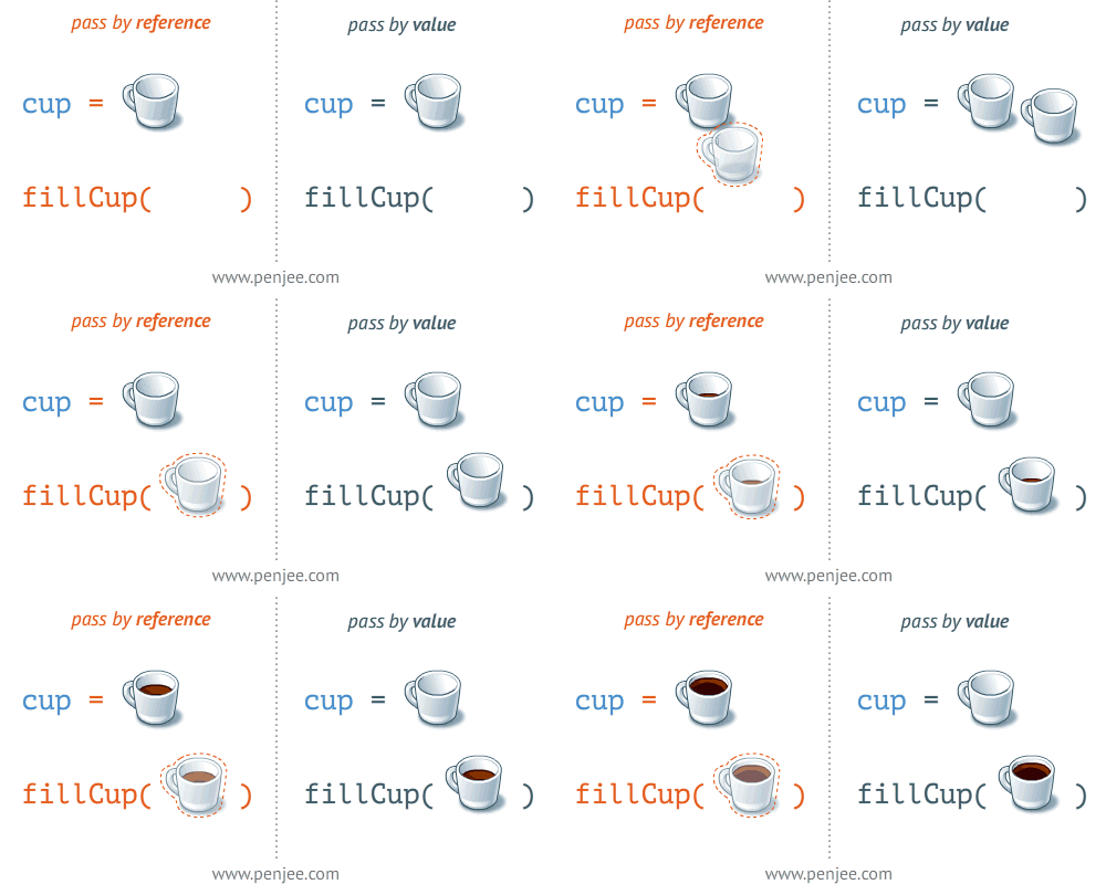
Passing by reference is akin to sending the URL to an object like a variable. This is usually done for big elements like a list or a plot. The caller and callee use the same variable.
Passing by parameter makes a whole separate copy (e.g. integers, strings, booleans, floats). The caller and callee both get an independent copy. I found an excellent visualization that sums it up nicely:
Garbage Collection - Heaps and Stacks.
Stack is used for static memory allocation. It is optimized quite closely by the CPU and you do not need to do any memory management. Stack variables are local in nature and are deleted after a function executes. Size is limited and variables cannot be resized.
Heaps are used for dynamic memory allocation that you have to manage carefully. It is a larger floating region of memory. You have to allocate it to use it, and deallocate it when you are done. Memory leak may occur if not properly deallocated. Heap variables are global in nature.
In python, you never have to worry about memory as it is automatically managed for you. The downside is some loss in speed
# Garbage collector in python
a=[1,2,3,4]
a='new string'
# the list 'a' is now unreferenced is garbage collected
APPENDIX B - Styling Recommendation
For styling and standard formatting of your code. Refer to PEP 8: Python Style Guide. You don’t need to follow the guideline exactly. But abiding by some of the rules here greatly improves readability. Some of the more common guidelines:
Recommended Boiler Plate Starter File
# Imports
import numpy as np
import time

# Constants
PI = 3.1415926
FILE_PATH = r"C:\Users\username\Desktop"

def main():
    """Start your code here"""
    pass


def my_helper_function():
    pass


# Boiler plate. No need to modify
if __name__ == "__main__":
    time_start = time.time()
    main()
    time_end = time.time()
    print("Script completed. Total elapsed time: {:.2f} seconds".format(time_end - time_start))
else:
    print("{} Package imported!".format(__name__))
Basics
# Always use 4-space indentation. Never mix & match. Most editors have options
# to convert tab to 4 spaces
	# Tab indentation
    # 4-space indentation

# Blank line separation: 2 for functions, 1 for methods. Use lines in code
# for logical sections (sparingly)

# Try to limit line length to ~80 characters if possible. Don't go over 120
#000000000000000000000000000000000000000000000000000000000000000000000000000000
#0000000000000000000000000000000000000000000000000000000000000000000000000000000000000000000000000000000

# Comments start with space and capital letter
myvar = 1 # Inline comment can be distracting
Common
# Don't compare boolean values to True or False
if boolean:
    print("Don't do boolean == True or False")

# Constants should be in all caps
MYCONSTANT = 3.14

# Naming convention for variables
a = "single letter for simple variables"
lowercase = "most optimal choice"
_ = "underscore usually used for temp variable that you have no interest in"

# For more descriptive variable name: (don't make too long)
lowercase = "used for module or function names"
lower_case_with_underscore = "used for function names"
CapWordStyle = "used for class names"
mixedCase = "usually dont use"

# There are too many arguments
myfunction(argument1, argument2, argument3, argument4, argument5,
           argument6, argument7, argument8, argument9, argument10)

# Defining a matrix
np.array([
    [1,2,3],
    [4,5,6]
])

# Usually have blank space after comma or math operator. Not always
a = income + 3*(a + n) - 3
b = c
somelist = [a, b, c, d]
Docstring standard
def myfunction(arg1,arg2):
    """Single-line docstring. Do something and return value a"""
    return a

class myclass
    """
    Multi-line docstring for more complex functions or classes. Provide a
    concise summary of the behavior. For classes list out the public methods
    and instance variables.
    Args:
    	parameter1:
    	parameter2:
    Returns:
    	Description of what is returned
    """
    return a

def function_with_doctest(a,b):
  """
  >>> function_with_doctest(2,3)
  6
  >>> function_with_doctest("a",3)
  "aaa"
  """
  return a*b
  # run this doc test in console by: py -m doctest -v filewithfunction.py
RANDOM NOTES
I put random notes here. Pretty much anything I found helpful can appear here. Slowly they will migrate to the other sections
# Open a website and read its content to a string (bypassing 403 forbidden)
# Simpler method is to use urllib.request.urlretrieve('example.com', 'test.txt')
import urllib.request
site= "https://ikea-status.dong.st/latest.json"
user_agent = 'Mozilla/5.0 (Windows; U; Windows NT 5.1; en-US; rv:1.9.0.7) Gecko/2009021910 Firefox/3.0.7'
headers={'User-Agent':user_agent,}
request=urllib.request.Request(site,None,headers) #The assembled request
response = urllib.request.urlopen(request)
myfile = response.read()
data=str(myfile)


# Convert time zone
#convert from gmt to pst
PST = GMT - datetime.timedelta(hours = 7)

#Loop for 30 seconds:
import time
t_end = time.time() + 60 * 15
while time.time() < t_end:
    pass

#make beeping sound:
import winsound
winsound.Beep(2500, 1000)


#Sending email
# make an unsecure gmail account first
import smtplib
import ssl
    port = 465
    address = 'test1@gmail.com'
    password = 'putyourpasswordhere'
    context = ssl.create_default_context()

    sender_email = address
    receiver_email = 'test@gmail.com'
    subject = 'Ikea Click & Collect Available' + ' at ' + store + '| Time: ' + currentTime
    text = 'mail generated via python'
    message = "Subject: {}\n\n{}".format(subject, text)

    with smtplib.SMTP_SSL("smtp.gmail.com", port, context=context) as server:
        server.login(address, password)
        server.sendmail(sender_email, receiver_email, message)


# Working with word documents
'''
Document Object -> paragraph Object -> Run Object
Run object are collection of words. Within a paragraph, there might be several
run object because any change in styling creates a new run.
'''
pip install python-docx
import docx

def getText(filename):
    doc = docx.Document(filename)
    fullText=[]
    for paragraph in doc.paragraphs:
        fullText.append(paragraph.text)
Comments